Advanced examples#

How to use Qibocal as a library#

Qibocal also allows executing protocols without the standard interface.

In the following tutorial we show how to run a single protocol using Qibocal as a library. For this particular example we will focus on the single shot classification protocol.

from qibocal.protocols.characterization import Operation
from qibolab import create_platform

# allocate platform
platform = create_platform("....")
# get qubits from platform
qubits = platform.qubits

# we select the protocol
protocol = Operation.single_shot_classification.value

protocol is a Routine object which contains all the necessary methods to execute the experiment.

In order to run a protocol the user needs to specify the parameters. The user can check which parameters need to be provided either by checking the documentation of the specific protocol or by simply inspecting protocol.parameters_type. For single_shot_classification we can pass just the number of shots in the following way:

parameters = experiment.parameters_type.load(dict(nshots=1024))

After defining the parameters, the user can perform the acquisition using experiment.acquisition which accepts the following parameters:

params (experiment.parameters_type): input parameters for the experiment
platform (qibolab.platform.Platform): Qibolab platform class
targets (Union[list[QubitId],list[QubitPairId], list[list[QubitId]]]) list with qubits where the acquisition will run

and returns the following:

data (experiment.data_type): data acquired
acquisition_time (float): acquisition time on hardware

data, acquisition_time = experiment.acquisition(params=parameters, platform=platform, qubits=qubits)

The user can now use the raw data acquired by the quantum processor to perform an arbitrary post-processing analysis. This is one of the main advantages of this API compared to the cli execution.

The fitting corresponding to the experiment (experiment.fit) can be launched in the following way:

fit, fit_time = experiment.fit(data)

To be more specific the user should pass as input data which is of type experiment.data_type and the outputs are the following:

fit: (experiment.results_type) input parameters for the experiment
fit_time (float): post-processing time

It is also possible to access the plots and the tables generated in the report using experiment.report which accepts the following parameters:

data: (experiment.data_type) data structure used by experiment
target (dict[QubitId, QubitPairId]): qubit / qubit pair to be plotted
fit: (experiment.results_type): data structure for post-processing used by experiment

# Plot for qubit 0
target = 0
figs, html_content = experiment.report(data=data, target=target, fit=fit)

experiment.report returns the following:

figs: list of plotly figures
html_content: raw html with additional information usually in the form of a table

In our case we get the following figure for qubit 0:

figs[0]

and we can render the html content in the following way:

import IPython
IPython.display.HTML(html_content)

How to add a new protocol#

In this tutorial we show how to add a new protocol to Qibocal.

Protocol implementation in `Qibocal`#

Currently, characterization/calibration protocols are divided in three steps: acquisition, fit and plot. Qibocal provides three data structures input parameters, data acquired and results, that collect all the information concerning the routine.

The relationship between steps and data structures are summarized in the following bullets:

acquisition receives as input parameters and outputs data
fit receives as input data and outputs results
plot receives as input data and results to visualize the protocol

This approach is flexible enough to allow the data acquisition without performing a post-processing analysis.

Step by step tutorial#

All protocols are located in ``src/qibocal/protocols/characterization <https://github.com/qiboteam/qibocal/tree/main/src/qibocal/protocols/characterization>``_. Suppose that we want to code a protocol to perform a RX rotation for different angles.

We create a file rotate.py in src/qibocal/protocols/characterization.

Parameters#

First, we define the input parameters.

from dataclasses import dataclass
from ...auto.operation import Parameters

@dataclass
class RotationParameters(Parameters):
    """Parameters for rotation protocol."""

    theta_start: float
    """Initial angle."""
    theta_end: float
    """Final angle."""
    theta_step: float
    """Angle step."""
    nshots: int
    """Number of shots."""

In this case you define a range for the angle to be probed alongside the number of shots.

Note

It is advised to use dataclasses. If you are not familiar have a look at the official documentation.

Data structure#

Secondly, we define a data structure that aims at storing both the angles and the probabilities measured for each qubit. A generic data structure is usually composed of some raw data (the data attribute), which is usually coded as a dictionary of arrays plus additional information if required.

import numpy as np
import numpy.typing as npt
from dataclasses import dataclass, field
from ...auto.operation import Data

RotationType = np.dtype([("theta", np.float64), ("prob", np.float64)])

@dataclass
class RotationData(Data):
    """Rotation data."""

    data: dict[QubitId, npt.NDArray[RotationType]] = field(default_factory=dict)
    """Raw data acquired."""

    def register_qubit(self, qubit, theta, prob):
        """Store output for single qubit."""
        ar = np.empty((1,), dtype=RotationType)
        ar["theta"] = theta
        ar["prob"] = prob
        if qubit in self.data:
            self.data[qubit] = np.rec.array(np.concatenate((self.data[qubit], ar)))
        else:
            self.data[qubit] = np.rec.array(ar)

Note

When the protocols will be executed the data will be saved automatically. The data attribute will be stored as a npz file, while the rest of the information will be stored as json file. If the user would like to use a custom format the implementation of a save method inside the data structure will be necessary.

Acquisition function#

In the acquisition function we are going to perform the experiment.

Note

A generic acquisition function must have the following signature

from qibolab.platform import Platform
from qibolab.qubits import QubitId,, QubitPairId
from typing import Union

def acquisition(params: RoutineParameters, platform: Platform, targets: Union[list[QubitId], list[QubitPairId], list[list[QubitId]]]) -> RoutineData
"""A generic acquisition function."""

from qibolab.platform import Platform
from qibolab.qubits import QubitId

def acquisition(
    params: RotationParameters,
    platform: Platform,
    targets: list[QubitId],
) -> RotationData:
    r"""
    Data acquisition for rotation routine.

    Args:
        params (:class:`RotationParameters`): input parameters
        platform (:class:`Platform`): Qibolab's platform
        targets (list): list with target qubits

    Returns:
        data (:class:`RotationData`)
    """

    # costruct range from RotationParameters
    angles = np.arange(params.theta_start, params.theta_end, params.theta_step)
    # create data structure
    data = RotationData()

    # create and execute circuit for each angle
    for angle in angles:

        circuit = Circuit(platform.nqubits)
        for qubit in qubits:
            circuit.add(gates.RX(qubit, theta=angle))
            circuit.add(gates.M(qubit))

        result = circuit(nshots=params.nshots)

        for qubit in qubits:

            # extract probability of 0
            prob = result.probabilities(qubits=[qubit])[0]
            # store measurements in Rotation Data
            data.register_qubit(qubit, theta=angle, prob=prob)

    return data

Result class#

Here we decided to code a generic Results that contains the fitted parameters for each qubit.

from qibolab.qubits import QubitId

@dataclass
class RotationResults(Results):
    """Results object for data"""
    fitted_parameters: dict[QubitId, list] = field(default_factory=dict)

Note

To check whether fitted parameters for a specific Qubit it might be necessary to re-write the __contains__ method if the Results inheritance include non-dictionary attributes.

Fit function#

The following function performs a sinusoidal fit for each qubit.

Note

A generic fit function must have the following signature
def fit(data: RoutineData) -> RoutineResults
""" A generic fit."

where Qubits is a dict[QubitId, Qubit].

from scipy.optmize import curve_fit

def fit(data: RotationData) -> RotationResults:

    qubits = data.qubits
    freqs = {}
    fitted_parameters = {}

    def cos_fit(x, offset, amplitude, omega):
        return offset + amplitude * np.cos(omega*x)

    for qubit in qubits:
        qubit_data = data[qubit]
        thetas = qubit_data.theta
        probs = qubit_data.prob

        popt, _ = curve_fit(cos_fit, thetas, probs)

        freqs[qubit] = popt[2] / 2*np.pi
        fitted_parameters[qubit]=popt.tolist()

    return RotationResults(
        fitted_parameters=fitted_parameters,
    )

Report function#

The report function generates a list of figures and an optional table to be shown in the html report. For the plotting function the user must use plotly in order to properly generate the report.

Note

A generic report function must have the following signature

import plotly.graph_objects as go

def plot(data: RoutineData, fit: RoutineResults, target: QubitId) -> list[go.Figure(), str]
""" A generic plotting function."""

The str in output can be used to create a table, which has 3 columns target, Fitting Parameter and Value. Here is the syntax necessary to insert a raw in the table.

report = ""
target = 0
angle = 3.14
report += f" {qubit} | rotation angle: {angle:.3f}<br>"

This table can be omitted by returnig None.

Here is the plotting function for the protocol that we are coding:

import plotly.graph_objects as go
from qibolab.qubits import QubitId

def plot(data: RotationData, fit: RotationResults, target: QubitId):
"""Plotting function for rotation."""

    figures = []
    fig = go.Figure()

    fitting_report = ""
    qubit_data = data[target]

    fig.add_trace(
        go.Scatter(
            x=qubit_data.theta,
            y=qubit_data.prob,
            opacity=1,
            name="Probability",
            showlegend=True,
            legendgroup="Voltage",
        ),
    )

    if fit is not None:
        fig.add_trace(
            go.Scatter(
                x=qubit_data.theta,
                y=cos_fit(
                    qubit_data.theta,
                    *fit.fitted_parameters[target],
                ),
                name="Fit",
                line=go.scatter.Line(dash="dot"),
            ),
        )

    # last part
    fig.update_layout(
        showlegend=True,
        xaxis_title="Theta [rad]",
        yaxis_title="Probability",
    )

    figures.append(fig)

    return figures, fitting_report

Create `Routine` object#

rotation = Routine(acquisition, fit, plot)
"""Rotation Routine  object."""

Add routine to Operation Enum#

The last step is to add the routine that we just created to the Operation Enum in src/qibocal/protocols/characterization/__init__.py:

# other imports...
from rotate import rotation


class Operation(Enum):
### other protocols...
rotation = rotation

Write a runcard#

To launch the protocol a possible runcard could be the following one:

platform: dummy

targets: [0,1]


actions:
    - id: rotate

      operation: rotation
      parameters:
        theta_start: 0
        theta_end: 7
        theta_step: 20
        nshots: 1024

For more information about how to execute runcards see How to execute calibration protocols in Qibocal?.

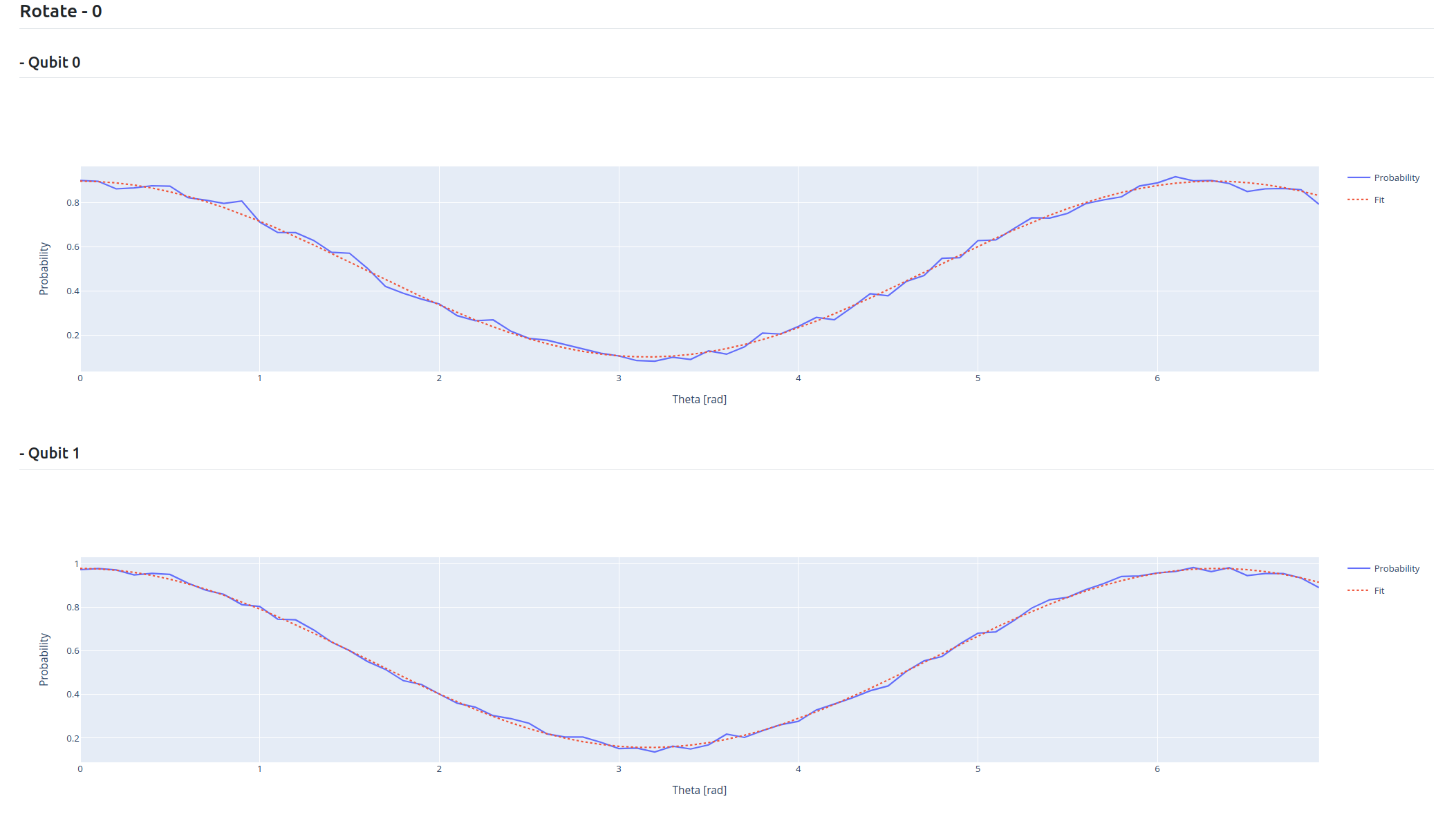
Here is the expected output:

Advanced examples#

How to use Qibocal as a library#

How to add a new protocol#

Protocol implementation in Qibocal#

Step by step tutorial#

Parameters#

Data structure#

Acquisition function#

Result class#

Fit function#

Report function#

Create Routine object#

Add routine to Operation Enum#

Write a runcard#

Protocol implementation in `Qibocal`#

Create `Routine` object#