Resonator spectroscopy#

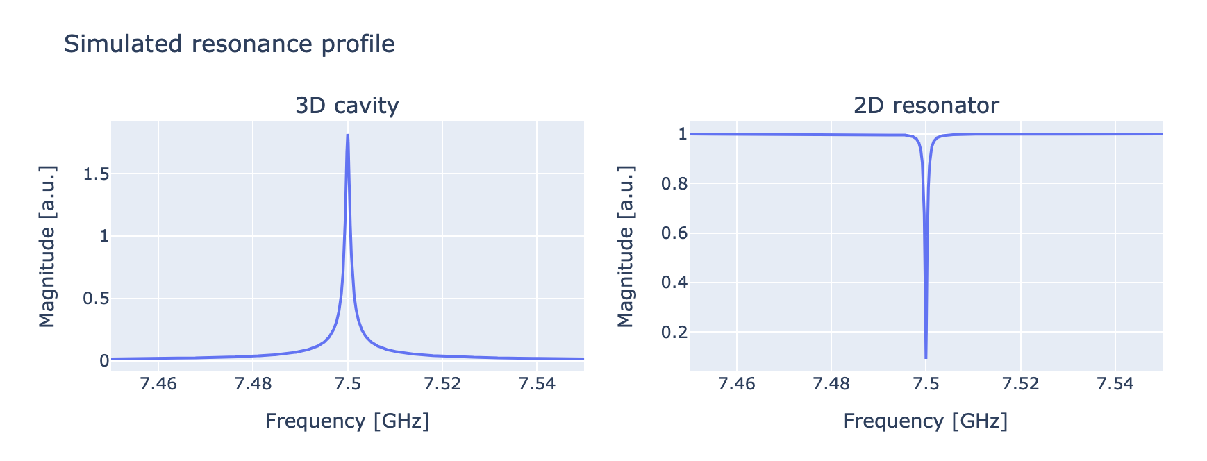
When calibrating the readout pulse, the first step is to identify the resonator frequency. At this frequency, we can observe a clear difference in the transmitted signal: for a 3D cavity resonator, an amplified signal will be observed, whereas for a 2D resonator, higher absorption will be spotted. In both cases, a Lorentzian peak is expected, which will be positive for 3D cavities and negative for 2D resonators.

In the experiment, we send a readout pulse with a fixed duration and amplitude. After waiting for the time of flight, we acquire and average a waveform, resulting in a single point.

Parameters#

class qibocal.protocols.resonator_spectroscopy.ResonatorSpectroscopyParameters(freq_width: int, freq_step: int, power_level: Union[PowerLevel, str], fit_function: str = 'lorentzian', phase_sign: bool = True, amplitude: Optional[float] = None, attenuation: Optional[int] = None, hardware_average: bool = True)[source]

ResonatorSpectroscopy runcard inputs.

freq_width: int: Width for frequency sweep relative to the readout frequency [Hz].

freq_step: int: Frequency step for sweep [Hz].

power_level: Union[PowerLevel, str]: Power regime (low or high). If low the readout frequency will be updated. If high both the readout frequency and the bare resonator frequency will be updated.

fit_function: str = 'lorentzian': Routine function (lorentzian or s21) to fit data with a model.

phase_sign: bool = True: Several instruments have their convention about the sign of the phase. If True, the routine will apply a minus to the phase data.

amplitude: Optional[float] = None: Readout amplitude (optional). If defined, same amplitude will be used in all qubits. Otherwise the default amplitude defined on the platform runcard will be used

attenuation: Optional[int] = None: Readout attenuation (optional). If defined, same attenuation will be used in all qubits. Otherwise the default attenuation defined on the platform runcard will be used

hardware_average: bool = True: By default hardware average will be performed.

nshots: int: Number of executions on hardware.

relaxation_time: float: Wait time for the qubit to decohere back to the gnd state.

This experiment is highly dependent on the pulse amplitude. The primary goal is to determine the resonator frequency without any readout optimization, which will be addressed later. For this purpose, we can fix the pulse duration to the order of magnitude of microseconds. The discussion regarding amplitude is more complex and involves several considerations:

higher amplitudes usually correspond to a better signal-to-noise ratio;
at high amplitudes the signal breaks superconductivity, therefore resonator is not effectively not coupled to the qubit (we talk of bare resonator frequency);
at intermediate amplitudes the peak could completely disappear and is, in general, not Lorentzian;
very high amplitudes could damage the components.

The bare resonator frequency can be found by setting a large value for the amplitude, e.g.:

Example#

- id: resonator_spectroscopy high power

  operation: resonator_spectroscopy
  parameters:
      freq_width: 60_000_000
      freq_step: 200_000
      amplitude: 0.6
      power_level: high
      nshots: 1024
      relaxation_time: 100000

Note

The resonator spectroscopy experiment will be performed by computing the average on hardware. If the user wants to retrieve all the shots and perform the average afterward it can be done by specifying the entry hardware_average: false in the experiment parameters. In this case, the fitting procedure will consider errors and error bands will be included in the plot.

../../_images/resonator_spectroscopy_error_bars.png

../../_images/resonator_spectroscopy_high.png

Lowering the amplitude we can see a shift in the peak, e.g.:

Example#

- id: resonator_spectroscopy low power

  operation: resonator_spectroscopy
  parameters:
      freq_width: 60_000_000
      freq_step: 200_000
      amplitude: 0.03
      power_level: low
      nshots: 1024
      relaxation_time: 100000

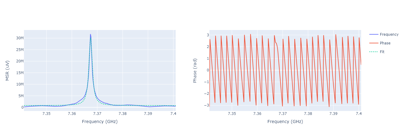
../../_images/resonator_spectroscopy_low.png

Running the qibocal routines above produces outputs in the reports like the ones shown above. The peaks are Lorentzian. However, a better description for a 2D notch resonator resonance profile is provided by [6, 13] where the complex signal is modeled as

\[S_{21}(f) = ae^{i\alpha}e^{-2\pi i f \tau}\left[ 1 - \frac{(Q_l/|Q_c|)e^{i\phi}}{1 + 2iQ_l(f/f_r -1)} \right]\]

This description gives insightful information, the first part describes the environment which involves:

\(a\): amplitude resulting from the attenuation and gain in the measurement system;
\(\alpha\): phase-shift associated with \(a\);
\(\tau\): cable delay caused by the length of the cable and the finite speed of light.

The second part describes the resonance of an ideal 2D notch resonator:

\(Q_l\): loaded (total) quality factor;
\(Q_c\): coupling (external) quality factor;
\(\phi\): accounts for impedance mismatches or reflections in cables (Fano interferences);
\(f_r\): resonance frequency.

The routine should be preferred over the Lorentzian fit because it exploits all the information in a signal, including both magnitude and phase. Nonetheless, performing a direct fit for all seven parameters simultaneously involves handling a nonlinear multi-parameter fitting problem, which is non-robust and extremely sensitive to the initial values. Therefore, the problem is divided into several independent fitting tasks to enhance robustness and accuracy:

Cable delay correction: the cable delay titls the phase signal by a slope \(2\pi\tau\) and to get a rough estimate, it is sufficient to fit a linear function to the phase signal. Without any cable delay, the resonance looks like a circle in the complex plane but the cable delay deforms this circle to a loop-like curve.
Circle fit: the center and radius of the circle resulting from the previous step are evaluated. The routine expolits the methods described in [5]. The data are shifted to the found center.
Phase fit: the phase angle \(\theta\) of the centered data as a function of frequency is fit with the following profile

\[\theta = \theta_0 - 2\pi \tau (f-f_r) + 2 \arctan \left[2 Q_r \left( 1 - \frac{f}{f_r} \right) \right]\]

The linear background slope accounts for an additional residual delay \(2\pi\tau(f - f_r)\), introducing an extra degree of freedom to the parameter set. Parameter estimation is performed through an iterative least squares process to optimize the model parameters.

Example#

- id: resonator_spectroscopy low power

  operation: resonator_spectroscopy
  parameters:
      freq_width: 20_000_000
      freq_step: 100_000
      amplitude: 0.01
      power_level: low
      nshots: 1024
      relaxation_time: 100_000
      fit_function: "s21"

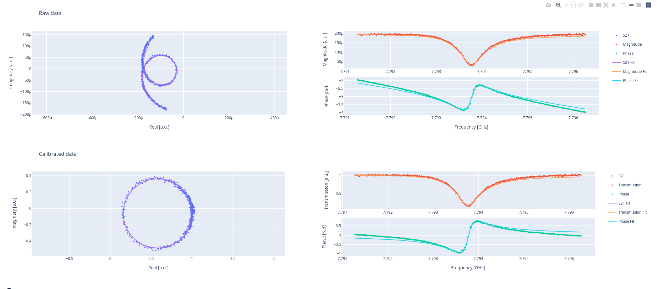
Note

The s21 routine provides a comprehensive report of the calibration and parameter estimation process. In the first row, the raw data are shown in the complex plane, typically distributed as a loop-like curve. To the right, the magnitude and phase of the signal of interest are presented. In the second row, after removing the environmental effects, the calibrated data are displayed, which should be approximately distributed as a circle in the complex plane.

Example#

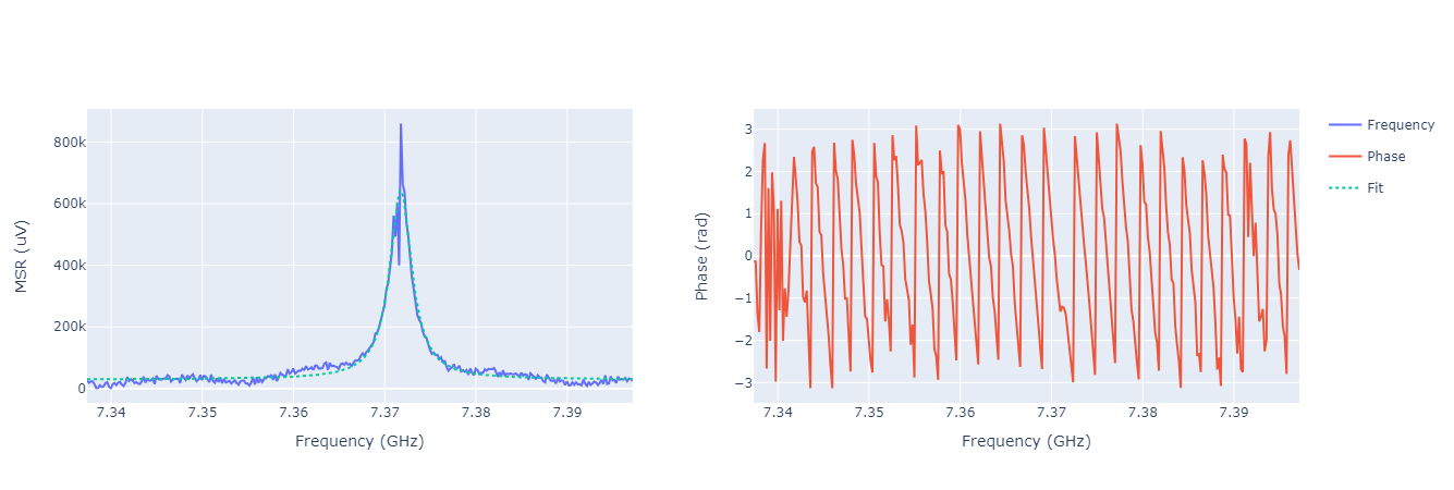
As expected, at low power the resonator frequency shifts. This is due to the Hamiltonian of the system [3, 14]. Therefore, the dressed resonator frequency is larger than the bare resonator frequency.

Lowering the amplitude value also reduces the height of the peak and increases the noise.

Another parameter connected to the amplitude, is also the relaxation time (in some literature also referred to as repetition duration) and the number of shots. The number of shots represents the number of repetitions of the same experiment (at the same frequency), while the relaxation time is the waiting time between repetitions. A higher number of shots will increase the S/N ratio by averaging the noise, but will also slow down the acquisition. As per the relaxation time, for this experiment in particular we can leave it at zero: since we are not exciting the qubit we do not particularly care about it. However note that, for 3D cavities, we could end up damaging the qubit if we send too much energy over a small period of time so it could be worth increasing the relaxation time. However, some electronics do not support zero relaxation times, therefore a relaxation time greater than zero is a safer choice.

Last but not least, we have to choose which frequencies are probed during the scan: a very wide scan can be useful if nothing is known about the studied resonator, but in general, we have at least the design parameters. These are often not exact but can give an idea of the region to scan (for standard cavities around 7 GHz). Also, a very small step between two subsequent frequency points is not needed and could really slow down the experiment (from seconds to tens of minutes) if chosen incorrectly. Usually, a step of 200 MHz is fine enough.

The resonator frequencies can be then inserted into the platform runcards (in qibolab_platforms_qrc). For example, if we are reading qubit 0:

native_gates:
    single_qubit:
        0: # qubit number
            RX:
                duration: 40
                amplitude: <high_power_amplitude>
                frequency: <high_power_resonator_frequency>
                shape: Gaussian(5)
                type: qd # qubit drive
                relative_start: 0
                phase: 0
            MZ:
                duration: 2000
                amplitude: <low_power_amplitude>
                frequency: <low_power_resonator_frequency>
                shape: Rectangular()
                type: ro # readout
                relative_start: 0
                phase: 0

and also here:

characterization:
    single_qubit:
        0:
            bare_resonator_frequency: <high_power_resonator_frequency>
            readout_frequency: <low_power_resonator_frequency>

Requirements#

Time Of Flight (Readout)