Qubit spectroscopies
In this section we are going to present how to run with qibocal some qubit spectroscopy experiments.
Qubit Spectroscopy
To measure the resonance frequency of the qubit it is possible to perform a qubit spectroscopy experiment. After having obtained an initial guess for the readout amplitude and the readout frequency through a Resonator punchout this experiment aims at extracting the frequency of the qubit.
In this protocol the qubit is probed by sending a drive pulse at variable frequency \(w\) before measuring. When \(w\) is close to the transition frequency \(w_{01}\) some of the population will move to the excited state. If the drive pulse is long enough it will be generated a maximally mixed state with \(\rho \propto I\) [2, 9].
Parameters
- class qibocal.protocols.qubit_spectroscopies.qubit_spectroscopy.QubitSpectroscopyParameters(freq_width: int, freq_step: int, drive_duration: int, drive_amplitude: float | None = None, hardware_average: bool = True)[source]
QubitSpectroscopy runcard inputs.
- freq_width: int
Width [Hz] for frequency sweep relative to the qubit frequency.
- freq_step: int
Frequency [Hz] step for sweep.
- drive_duration: int
Drive pulse duration [ns]. Same for all qubits.
- hardware_average: bool = True
By default hardware average will be performed.
- nshots: int
Number of executions on hardware.
- relaxation_time: float
Wait time for the qubit to decohere back to the gnd state.
How to execute a qubit spectroscopy experiment
A possible runcard to launch a qubit spectroscopy experiment could be the following:
- id: qubit spectroscopy 01
  operation: qubit_spectroscopy
  parameters:
    drive_amplitude: 0.01 # drive power
    drive_duration: 4000 # ns
    freq_width: 20_000_000
    freq_step: 1_000_000
    nshots: 1024
    relaxation_time: 20_000
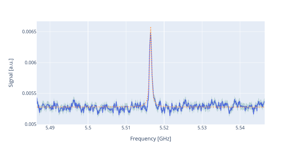
Here is the corresponding plot:

To extract the qubit frequency a Lorentzian fit is performed.
Requirements
Qubit spectroscopy for higher excited states
Through a qubit spectroscopy experiment it is possible to target also the transition frequencies towards higher energy level other than the first excited state.
To visualize these secondary excitations it is necessary to provide a considerable amount of drive power, which might be outside the limit of the experimental setup.
Another way to address the higher levels is to first excite the qubit to state \(\ket{1}\) followed by the sequence previously presented for the qubit spectroscopy. In this way it is possible to induce a transition between \(\ket{1}\leftrightarrow\ket{2}\).
Such frequency \(\omega_{12}\) should be below \(\omega_{01}\) by around \(200 - 300\) MHz for flux tunable transmons. From \(\omega_{12}\) and \(\omega_{01}\) it is possible to compute the anharmonicity \(\alpha\) as [14]:
In the literature the energy levels can be expressed as \(\ket{g}, \ket{e}, \ket{f}\), to
address the ground state, the excited state and the first excited state above the excited state.
For this reason the experiments has been labelled qubit_spectroscopy_ef.
Parameters
- class qibocal.protocols.qubit_spectroscopies.qubit_spectroscopy_ef.QubitSpectroscopyEFParameters(freq_width: int, freq_step: int, drive_duration: int, drive_amplitude: float | None = None, hardware_average: bool = True)[source]
QubitSpectroscopyEF runcard inputs.
- hardware_average: bool = True
By default hardware average will be performed.
- freq_width: int
Width [Hz] for frequency sweep relative to the qubit frequency.
- freq_step: int
Frequency [Hz] step for sweep.
- drive_duration: int
Drive pulse duration [ns]. Same for all qubits.
- nshots: int
Number of executions on hardware.
- relaxation_time: float
Wait time for the qubit to decohere back to the gnd state.
How to execute a qubit spectroscopy experiment
A possible runcard to launch a qubit spectroscopy experiment could be the following:
- id: qubit spectroscopy 12
  operation: qubit_spectroscopy_ef
  parameters:
    drive_amplitude: 0.01 # drive power
    drive_duration: 4000 # ns
    freq_width: 20_000_000
    freq_step: 1_000_000
    nshots: 1024
    relaxation_time: 20_000
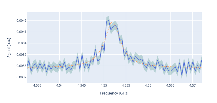
Here is the corresponding plot:

To extract \(\omega_{12}\) a lorentzian fit is performed. After the post-processing both the anharmonicity and the frequency of the RX12 pulse (which is the pulse that allows to drive a qubit from state \(\ket{1}\) to state \(\ket{2}\)) are updated.