Models#

Qibo provides models for both the circuit based and the adiabatic quantum computation paradigms. Circuit based models include Circuit models which allow defining arbitrary circuits and Quantum Fourier Transform (QFT) such as the Quantum Fourier Transform (qibo.models.QFT) and the Variational Quantum Eigensolver (qibo.models.VQE). Adiabatic quantum computation is simulated using the Time evolution of state vectors.

In order to perform calculations and apply gates to a state vector a backend has to be used. The backends are defined in qibo/backends. Circuit and gate objects are backend independent and can be executed with any of the available backends.

Qibo uses big-endian byte order, which means that the most significant qubit is the one with index 0, while the least significant qubit is the one with the highest index.

Circuit models#

Circuit#

class qibo.models.circuit.Circuit(nqubits=None, accelerators=None, density_matrix=False, wire_names=None)[source]#

Circuit object which holds a list of gates.

This circuit is symbolic and cannot perform calculations. A specific backend has to be used for performing calculations.

Circuits can be created with a specific number of qubits and wire names.

Either nqubits or wire_names must be provided.

If only nqubits is provided, wire names will default to [0, 1, ..., nqubits - 1].

If only wire_names is provided, nqubits will be set to the length of wire_names.

nqubits and wire_names must be consistent with each other.

Example:

from qibo import Circuit

# Every circuit initialization below is valid
circuit = Circuit(5)  # Default wire names are [0, 1, 2, 3, 4]
circuit = Circuit(["A", "B", "C", "D", "E"])
circuit = Circuit(5, wire_names=["A", "B", "C", "D", "E"])
circuit = Circuit(wire_names=["A", "B", "C", "D", "E"])

Parameters:

nqubits (int | list | None) –
accelerators (dict | None) –
density_matrix (bool) –
wire_names (list | None) –

nqubits#

Number of qubits in the circuit or a list of wire names.

Type:: int | list, optional

wire_names#

List of wire names

Type:: list, optional

init_kwargs#

a dictionary with the following keys

nqubits
accelerators
density_matrix
wire_names.

Type:: dict

queue#

List that holds the queue of gates of a circuit.

Type:: _Queue

parametrized_gates#

List of parametric gates.

Type:: _ParametrizedGates

trainable_gates#

List of trainable gates.

Type:: _ParametrizedGates

measurements#

List of non-collapsible measurements.

Type:: list

_final_state#: Final result after full simulation of the circuit.

compiled#

Circuit executor. Defaults to None.

Type:: CompiledExecutor

repeated_execution#

If True, the circuit would be re-executed when sampling. Defaults to False.

Type:: bool

density_matrix#

If True, the circuit would evolve density matrices. If False, defaults to statevector simulation. Defaults to False.

Type:: bool, optional

accelerators#

Dictionary that maps device names to the number of times each device will be used. Defaults to None.

Type:: dict, optional

ndevices#

Total number of devices. Defaults to None.

Type:: int

nglobal#

Base two logarithm of the number of devices. Defaults to None.

Type:: int

nlocal#

Total number of available qubits in each device. Defaults to None.

Type:: int

queues#

Gate queues for each accelerator device. Defaults to None.

Type:: DistributedQueues

on_qubits(*qubits)[source]#

Generator of gates contained in the circuit acting on specified qubits.

Useful for adding a circuit as a subroutine in a larger circuit.

Parameters:: qubits (int) – Qubit ids that the gates should act.

Example

from qibo import Circuit, gates

# create small circuit on 4 qubits
small_circuit = Circuit(4)
small_circuit.add(gates.RX(qubit, theta=0.1) for qubit in range(4))
small_circuit.add((gates.CNOT(0, 1), gates.CNOT(2, 3)))
# create large circuit on 8 qubits
large_circuit = Circuit(8)
large_circuit.add(gates.RY(qubit, theta=0.1) for qubit in range(8))
# add the small circuit to the even qubits of the large one
large_circuit.add(small_circuit.on_qubits(*range(0, 8, 2)))

light_cone(*qubits)[source]#

Reduces circuit to the qubits relevant for an observable.

Useful for calculating expectation values of local observables without requiring simulation of large circuits. Uses the light cone construction described in issue #571.

Parameters:

qubits (int) – Qubit ids that the observable has support on.

Returns:

Circuit that contains only: the qubits that are required for calculating expectation involving the given observable qubits.
qubit_map (dict): Dictionary mapping the qubit ids of the original: circuit to the ids in the new one.

Return type:

circuit (qibo.models.Circuit)

copy(deep=False)[source]#

Creates a copy of the current circuit as a new Circuit model.

Parameters:: deep (bool) – If True copies of the gate objects will be created for the new circuit. If False, the same gate objects of circuit will be used.
Returns:: The copied circuit object.

invert()[source]#

Creates a new Circuit that is the inverse of the original.

Inversion is obtained by taking the dagger of all gates in reverse order. If the original circuit contains parametrized gates, dagger will change their parameters. This action is not persistent, so if the parameters are updated afterwards, for example using qibo.models.circuit.Circuit.set_parameters(), the action of dagger will be overwritten. If the original circuit contains measurement gates, these are included in the inverted circuit.

Returns:: Circuit corresponding to the inverse of the original circuit.
Return type:: qibo.models.Circuit

decompose(*free, method='standard', **kwargs)[source]#

Decomposes circuit’s gates to gates supported by OpenQASM.

Parameters:

free (int) – Ids of free (work) qubits that can be used as dirty auxiliary qubits in the decomposition of multi-controlled gates, that is, they can be in any state and are left unchanged. They must not be qubits that the decomposed gates act on.
method (str, optional) – Choice of gate set for the decomposition. If "standard", decomposes circuit into qibo.gates.gates.CNOT, qibo.gates.gates.RX, qibo.gates.gates.RY, qibo.gates.gates.RZ, qibo.gates.gates.U1, qibo.gates.gates.U2, qibo.gates.gates.U3, and Clifford gates. If "clifford_plus_t", decomposes the circuit into qibo.gates.gates.CNOT, qibo.gates.gates.H, qibo.gates.gates.S, qibo.gates.gates.X, qibo.gates.gates.Y, qibo.gates.gates.Z, and qibo.gates.gates.T. Defaults to "standard".
kwargs (dict, optional) – Additional arguments passed to qibo.gates.abstract.Gate.decompose() for each gate. For example, clean, minimize_toffolis and minimize_depth select other decompositions of multi-controlled gates.

Returns:

Circuit that contains only gates that are supported by OpenQASM and has the same effect as the original circuit.

Return type:

qibo.models.circuit.Circuit

with_pauli_noise(noise_map)[source]#

Creates a copy of the circuit with Pauli noise gates after each gate.

If the original circuit uses state vectors then noise simulation will be done using sampling and repeated circuit execution. In order to use density matrices the original circuit should be created setting the flag density_matrix=True. For more information we refer to the How to perform noisy simulation? example.

Parameters:: noise_map (dict) – list of tuples $(P_{k}, p_{k})$, where $P_{k}$ is a str representing the $k$-th $n$-qubit Pauli operator, and $p_{k}$ is the associated probability.
Returns:: Circuit object that contains all the gates of the original circuit and additional noise channels on all qubits after every gate.

Example

from qibo import Circuit, gates
# use density matrices for noise simulation
circuit = Circuit(2, density_matrix=True)
circuit.add([gates.H(0), gates.H(1), gates.CNOT(0, 1)])
noise_map = {
    0: list(zip(["X", "Z"], [0.1, 0.2])),
    1: list(zip(["Y", "Z"], [0.2, 0.1]))
}
noisy_circuit = circuit.with_pauli_noise(noise_map)
# ``noisy_circuit`` will be equivalent to the following circuit
circuit_2 = Circuit(2, density_matrix=True)
circuit_2.add(gates.H(0))
circuit_2.add(gates.PauliNoiseChannel(0, [("X", 0.1), ("Z", 0.2)]))
circuit_2.add(gates.H(1))
circuit_2.add(gates.PauliNoiseChannel(1, [("Y", 0.2), ("Z", 0.1)]))
circuit_2.add(gates.CNOT(0, 1))
circuit_2.add(gates.PauliNoiseChannel(0, [("X", 0.1), ("Z", 0.2)]))
circuit_2.add(gates.PauliNoiseChannel(1, [("Y", 0.2), ("Z", 0.1)]))

add(gate)[source]#

Add a gate to a given queue.

Parameters:: gate (qibo.gates.Gate) – the gate object to add. See Gates for a list of available gates. gate can also be an iterable or generator of gates. In this case all gates in the iterable will be added in the circuit.
Returns:: If the circuit contains measurement gates with collapse=True a sympy.Symbol that parametrizes the corresponding outcome.

property measurement_tuples: dict#: used for testing only

property ngates: int#: Total number of gates/operations in the circuit.

property depth: int#: Circuit depth if each gate is placed at the earliest possible position.

property gate_types: Counter#: collections.Counter with the number of appearances of each gate type.

property gate_names: Counter#: collections.Counter with the number of appearances of each gate name.

gates_of_type(gate)[source]#

Finds all gate objects of specific type or name.

This method can be affected by how qibo.gates.Gate.controlled_by() behaves with certain gates. To see how qibo.gates.Gate.controlled_by() affects gates, we refer to the documentation of qibo.gates.Gate.controlled_by().

Parameters:

gate (str or type) – The name of a gate or the corresponding gate class.

Returns:

gates that are in the circuit and have the same type as gate.: The list contains tuples (k, g) where k is the index of the gate g in the circuit’s gate queue.

Return type:

list

set_parameters(parameters)[source]#

Updates the parameters of the circuit’s parametrized gates.

For more information on how to use this method we refer to the How to use parametrized gates? example.

Parameters:: parameters (list[float] | dict[str, float] | _Buffer | _SupportsArray[dtype[Any]] | _NestedSequence[_SupportsArray[dtype[Any]]] | bool | int | float | complex | str | bytes | _NestedSequence[bool | int | float | complex | str | bytes]) – Container holding the new parameter values. It can have one of the following types: List with length equal to the number of parametrized gates and each of its elements compatible with the corresponding gate. Dictionary with keys that are references to the parametrized gates and values that correspond to the new parameters for each gate. Flat list with length equal to the total number of free parameters in the circuit. A backend supported tensor (for example np.ndarray or tf.Tensor) may also be given instead of a flat list.
Return type:: None

Example

from qibo import Circuit, gates
# create a circuit with all parameters set to 0.
circuit = Circuit(3)
circuit.add(gates.RX(0, theta=0))
circuit.add(gates.RY(1, theta=0))
circuit.add(gates.CZ(1, 2))
circuit.add(gates.fSim(0, 2, theta=0, phi=0))
circuit.add(gates.H(2))

# set new values to the circuit's parameters using list
params = [0.123, 0.456, (0.789, 0.321)]
circuit.set_parameters(params)
# or using dictionary
params = {
    circuit.queue[0]: 0.123,
    circuit.queue[1]: 0.456,
    circuit.queue[3]: (0.789, 0.321)
}
circuit.set_parameters(params)
# or using flat list (or an equivalent `np.array`/`tf.Tensor`/`torch.Tensor`)
params = [0.123, 0.456, 0.789, 0.321]
circuit.set_parameters(params)

get_parameters(output_format='list', include_not_trainable=False)[source]#

Returns the parameters of all parametrized gates in the circuit.

Inverse method of qibo.models.circuit.Circuit.set_parameters().

Parameters:

output_format (str) – Format to return the variational parameters. Available formats are "list", "dict" and "flatlist". See qibo.models.circuit.Circuit.set_parameters() for more details on each format. Default is "list".
include_not_trainable (bool) – If True it includes the parameters of non-trainable parametrized gates in the returned list or dictionary. Default is False.

Return type:

list | dict

associate_gates_with_parameters()[source]#

Associates to each parameter its gate.

Returns:: A nparams-long flatlist whose i-th element is the gate parameterized by the i-th parameter.
Return type:: list[qibo.gates.abstract.Gate]

summary_string()[source]#

Generate a summary of the circuit.

Return type:: str

summary()[source]#

Display a summary of the circuit.

The summary contains the circuit depths, total number of qubits and the all gates sorted in decreasing number of appearance.

Example:

from qibo import Circuit, gates

circuit = Circuit(3)
circuit.add(gates.H(0))
circuit.add(gates.H(1))
circuit.add(gates.CNOT(0, 2))
circuit.add(gates.CNOT(1, 2))
circuit.add(gates.H(2))
circuit.add(gates.TOFFOLI(0, 1, 2))

circuit.summary()

# Output:
# Circuit depth = 5
# Total number of gates = 6
# Number of qubits = 3
# Most common gates:
# h: 3
# cx: 2
# ccx: 1

Return type:: None

fuse(max_qubits=2)[source]#

Creates an equivalent circuit by fusing gates for increased simulation performance.

Parameters:: max_qubits (int) – Maximum number of qubits in the fused gates.
Returns:: A qibo.core.circuit.Circuit object containing qibo.gates.FusedGate gates, each of which corresponds to a group of some original gates. For more details on the fusion algorithm we refer to the Circuit fusion section.

Example

from qibo import Circuit, gates

circuit = Circuit(2)
circuit.add([gates.H(0), gates.H(1)])
circuit.add(gates.CNOT(0, 1))
circuit.add([gates.Y(0), gates.Y(1)])
# create circuit with fused gates
fused_circuit = circuit.fuse()
# now ``fused_circuit`` contains a single ``FusedGate`` that is
# equivalent to applying the five original gates

unitary(backend=None)[source]#

Creates the unitary matrix corresponding to all circuit gates.

This is a $2^{n} \times 2^{n}`$ matrix obtained by multiplying all circuit gates, where $n$ is nqubits.

Parameters:: backend (Backend | None) –
Return type:: _Buffer | _SupportsArray[dtype[Any]] | _NestedSequence[_SupportsArray[dtype[Any]]] | bool | int | float | complex | str | bytes | _NestedSequence[bool | int | float | complex | str | bytes]

Returns the final state after full simulation of the circuit.

If the circuit is executed more than once, only the last final state is returned.

execute(initial_state=None, nshots=1000, **kwargs)[source]#

Executes the circuit. Exact implementation depends on the backend.

Parameters:

initial_state (ndarray or qibo.models.circuit.Circuit) – Initial configuration. It can be specified by the setting the state vector using an array or a circuit. If None, the initial state is |000..00>.
nshots (int, optional) – Number of shots. Defaults ot $1000$.

Returns:

Either a qibo.result.QuantumState, qibo.result.MeasurementOutcomes or qibo.result.CircuitResult depending on the circuit’s configuration.

property raw: dict#

Serialize the circuit to a JSON-compatible dictionary.

This is a thin wrapper over qibo.gates.Gate.raw(). The returned dictionary has the following structure:

{
    "queue": [ <gate.raw>, ... ],  # list of serialized gates
    "nqubits": int,                # number of qubits
    "density_matrix": bool,        # whether a density matrix is used
    "wire_names": list | None,     # wire names (or None)
    "qibo_version": str,           # qibo version used for serialization
}

Each entry of queue is the output of qibo.gates.Gate.raw(). The dictionary can be loaded back into a circuit with qibo.models.circuit.Circuit.from_dict().

Returns:: JSON-compatible representation of the circuit.
Return type:: dict

classmethod from_dict(raw)[source]#

Load from serialization.

Essentially the counter-part of raw().

Parameters:: raw (dict) –

to_qasm(extended_compatibility=False)[source]#

Convert circuit to a QASM string.

Parameters:: extended_compatibility (bool) – if True, unrolls more exotic gates in their decomposition by defining them as custom gates, this increases the compatibility with other frameworks, such as qiskit. Defaults to False.
Returns:: The generated QASM.
Return type:: str

Note

This method does not support multi-controlled gates and gates with torch.Tensor as parameters.

to_qasm_file(qasm_file, extended_compatibility=False)[source]#

_summary_

Parameters:

qasm_file (str) – Path to file containing the QASM script.
extended_compatibility (bool, optional) – if True, unrolls more exotic gates in their decomposition by defining them as custom gates, this increases the compatibility with other frameworks, such as qiskit. Defaults to False.

Return type:

None

classmethod from_qasm(qasm_code, **circuit_kwargs)[source]#

Constructs a circuit from QASM code.

Parameters:

qasm_code (str) – String with the QASM script.
circuit_kwargs (dict) – Keyword arguments of the circuit.

Returns:

Circuit containing the gates specified by the given QASM script.

Return type:

qibo.models.circuit.Circuit

Example

from qibo import Circuit, gates
qasm_code = '''OPENQASM 2.0;
include "qelib1.inc";
qreg q[2];
h q[0];
h q[1];
cx q[0],q[1];'''
circuit = Circuit.from_qasm(qasm_code)
# is equivalent to creating the following circuit
circuit_2 = Circuit(2)
circuit_2.add(gates.H(0))
circuit_2.add(gates.H(1))
circuit_2.add(gates.CNOT(0, 1))

classmethod from_qasm_file(qasm_file, **circuit_kwargs)[source]#

Constructs a circuit from QASM code in a qasm_file.

Parameters:

qasm_file (str) – Path to file containing the string with the QASM script.
circuit_kwargs (dict) – Keyword arguments of the circuit.

Returns:

Circuit containing the gates specified by the given QASM script.

Return type:

qibo.models.circuit.Circuit

to_qir()[source]#

Convert circuit to QIR circuit.

Uses qbraid (https://github.com/qBraid/qBraid) to transpile the circuit into pyqir circuits.

to_cudaq()[source]#

Convert circuit to CUDA-Q (quake) code.

Uses qbraid (https://github.com/qBraid/qBraid) to transpile the circuit into cudaq circuits.

classmethod from_cudaq(cudaq_circuit_code)[source]#

Construct a circuit from CUDA-Q (quake) code.

Uses qbraid (https://github.com/qBraid/qBraid) to transpile the cudaq circuit into a qibo.models.circuit.Circuit.

Parameters:: cudaq_circuit_code (PyKernel) – kernel containing the cudaq circuit code.
Returns:: qibo.models.circuit.Circuit representing the given circuit.

diagram(line_wrap=100, legend=False, parallel=False)[source]#

Build the string representation of the circuit diagram.

See qibo.models.circuit.Circuit.draw() for the arguments.

Parameters:

line_wrap (int) –
legend (bool) –
parallel (bool) –

Return type:

str

draw(line_wrap=100, legend=False, parallel=False)[source]#

Draw text circuit using unicode symbols.

Parameters:

line_wrap (int, optional) – maximum number of characters per line. This option split the circuit text diagram in chunks of line_wrap characters. Defaults to $100$.
legend (bool, optional) – If True prints a legend below the circuit for callbacks and channels. Defaults to False.
parallel (bool, optional) – If True, multi-qubit gates acting on disjoint sets of wires are drawn in the same column, as single-qubit gates already are. A gate occupies every wire between its outermost qubits, so gates whose vertical connectors would cross are still drawn in separate columns. If False, each multi-qubit gate is drawn in its own column. Defaults to False.

Return type:

None

Circuit addition#

qibo.models.circuit.Circuit objects support addition. For example

circuit_1 = QFT(4)

circuit_2 = Circuit(4)
circuit_2.add(gates.RZ(0, 0.1234))
circuit_2.add(gates.RZ(1, 0.1234))
circuit_2.add(gates.RZ(2, 0.1234))
circuit_2.add(gates.RZ(3, 0.1234))

circuit = circuit_1 + circuit_2

will create a circuit that performs the Quantum Fourier Transform on four qubits followed by Rotation-Z gates.

Circuit fusion#

Gates in a circuit can be fused into a smaller number of qibo.gates.special.FusedGate objects using qibo.models.circuit.Circuit.fuse(). See Circuit fusion for a detailed description of the fusion algorithm and worked examples.

Quantum Fourier Transform (QFT)#

class qibo.models.qft.QFT(nqubits, with_swaps=True, accelerators=None, **kwargs)[source]#

Creates a circuit that implements the Quantum Fourier Transform.

Parameters:

nqubits (int) – number of qubits in the circuit.
with_swaps (bool, optional) – If True, uses qibo.gates.SWAP gates at the end of the circuit so that the qubit order in the final state is the same as the initial state. Defauts to True.
accelerators (dict, optional) – Accelerator device dictionary in order to use a distributed circuit. If None, a simple (non-distributed) circuit will be used.
kwargs (dict, optional) – Additional arguments used to initialize qibo.models.Circuit. For details, see the documentation of qibo.models.circuit.Circuit.

Returns:

implementation of the Quantum Fourier Transform.

Return type:

qibo.models.Circuit

Example

import numpy as np
from qibo.models import QFT
nqubits = 6
circuit = QFT(nqubits)
# Random normalized initial state vector
init_state = np.random.random(2 ** nqubits) + 1j * np.random.random(2 ** nqubits)
init_state = init_state / np.sqrt((np.abs(init_state)**2).sum())
# Execute the circuit
final_state = circuit(init_state)

Variational Quantum Eigensolver (VQE)#

class qibo.models.variational.VQE(circuit, hamiltonian)[source]#

This class implements the variational quantum eigensolver algorithm.

Parameters:

circuit (qibo.models.circuit.Circuit) – Circuit that implements the variaional ansatz.
hamiltonian (qibo.hamiltonians.Hamiltonian) – Hamiltonian object.

Example

import numpy as np

from qibo import Circuit, gates
from qibo.hamiltonians import XXZ
from qibo.models import VQE

# create circuit ansatz for two qubits
circuit = Circuit(2)
circuit.add(gates.RY(0, theta=0))
# create XXZ Hamiltonian for two qubits
hamiltonian = XXZ(2)
# create VQE model for the circuit and Hamiltonian
vqe = VQE(circuit, hamiltonian)
# optimize using random initial variational parameters
initial_parameters = np.random.uniform(0, 2, 1)
vqe.minimize(initial_parameters)

minimize(initial_state, method='Powell', loss_func=None, jac=None, hess=None, hessp=None, bounds=None, constraints=(), tol=None, callback=None, options=None, compile=False, processes=None)[source]#

Search for parameters which minimizes the hamiltonian expectation.

Parameters:

initial_state (array) – a initial guess for the parameters of the variational circuit.
method (str) – the desired minimization method. See qibo.optimizers.optimize() for available optimization methods.
loss (callable) – loss function, the default one is qibo.models.utils.vqe_loss().
jac (dict) – Method for computing the gradient vector for scipy optimizers.
hess (dict) – Method for computing the hessian matrix for scipy optimizers.
hessp (callable) – Hessian of objective function times an arbitrary vector for scipy optimizers.
bounds (sequence or Bounds) – Bounds on variables for scipy optimizers.
constraints (dict) – Constraints definition for scipy optimizers.
tol (float) – Tolerance of termination for scipy optimizers.
callback (callable) – Called after each iteration for scipy optimizers.
options (dict) – a dictionary with options for the different optimizers.
compile (bool) – whether the TensorFlow graph should be compiled.
processes (int) – number of processes when using the paralle BFGS method.

Returns:

The final expectation value. The corresponding best parameters. The optimization result object. For scipy methods it returns the OptimizeResult, for 'cma' the CMAEvolutionStrategy.result, and for 'sgd' the options used during the optimization.

energy_fluctuation(state)[source]#

Evaluate energy fluctuation

\[\Xi_{k}(\mu) = \sqrt{\langle\mu|\hat{H}^2|\mu\rangle - \langle\mu|\hat{H}|\mu\rangle^2} \,\]

for a given state $|\mu\rangle$.

Parameters:: state (np.ndarray) – quantum state to be used to compute the energy fluctuation with H.

Adiabatically Assisted Variational Quantum Eigensolver (AAVQE)#

class qibo.models.variational.AAVQE(circuit, easy_hamiltonian, problem_hamiltonian, s, nsteps=10, t_max=1, bounds_tolerance=1e-07, time_tolerance=1e-07)[source]#

This class implements the Adiabatically Assisted Variational Quantum Eigensolver algorithm. See https://arxiv.org/abs/1806.02287.

Parameters:

circuit (qibo.models.circuit.Circuit) – variational ansatz.
easy_hamiltonian (qibo.hamiltonians.Hamiltonian) – initial Hamiltonian object.
problem_hamiltonian (qibo.hamiltonians.Hamiltonian) – problem Hamiltonian object.
s (callable) – scheduling function of time that defines the adiabatic evolution. It must verify boundary conditions: s(0) = 0 and s(1) = 1.
nsteps (float) – number of steps of the adiabatic evolution.
t_max (float) – total time evolution.
bounds_tolerance (float) – tolerance for checking s(0) = 0 and s(1) = 1.
time_tolerance (float) – tolerance for checking if time is greater than t_max.

Example

import numpy as np

from qibo import Circuit, gates
from qibo.hamiltonians import X, XXZ
from qibo.models import AAVQE

# create circuit ansatz for two qubits
circuit = Circuit(2)
circuit.add(gates.RY(0, theta=0))
circuit.add(gates.RY(1, theta=0))
# define the easy and the problem Hamiltonians.
easy_hamiltonian = X(2)
problem_hamiltonian = XXZ(2)
# define a scheduling function with only one parameter
# and boundary conditions s(0) = 0, s(1) = 1
s = lambda t: t
# create AAVQE model
aavqe = AAVQE(
    circuit,
    easy_hamiltonian,
    problem_hamiltonian,
    s,
    nsteps=10,
    t_max=1
)
# optimize using random initial variational parameters
np.random.seed(0)
initial_parameters = np.random.uniform(0, 2*np.pi, 2)
ground_energy, params = aavqe.minimize(initial_parameters)

set_schedule(func)[source]#: Set scheduling function s(t) as func.

schedule(t)[source]#: Returns scheduling function evaluated at time t: s(t/Tmax).

hamiltonian(t)[source]#: Returns the adiabatic evolution Hamiltonian at a given time.

minimize(params, method='BFGS', jac=None, hess=None, hessp=None, bounds=None, constraints=(), tol=None, options=None, compile=False, processes=None)[source]#

Performs minimization to find the ground state of the problem Hamiltonian.

Parameters:

params (np.ndarray or list) – initial guess for the parameters of the variational circuit.
method (str) – optimizer to employ.
jac (dict) – Method for computing the gradient vector for scipy optimizers.
hess (dict) – Method for computing the hessian matrix for scipy optimizers.
hessp (callable) – Hessian of objective function times an arbitrary vector for scipy optimizers.
bounds (sequence or Bounds) – Bounds on variables for scipy optimizers.
constraints (dict) – Constraints definition for scipy optimizers.
tol (float) – Tolerance of termination for scipy optimizers.
options (dict) – a dictionary with options for the different optimizers.
compile (bool) – whether the TensorFlow graph should be compiled.
processes (int) – number of processes when using the parallel BFGS method.

Quantum Approximate Optimization Algorithm (QAOA)#

class qibo.models.variational.QAOA(hamiltonian, mixer=None, solver='exp', callbacks=None, accelerators=None)[source]#

Quantum Approximate Optimization Algorithm (QAOA) model.

The QAOA is introduced in arXiv:1411.4028.

Parameters:

hamiltonian (qibo.hamiltonians.Hamiltonian) – problem Hamiltonian whose ground state is sought.
mixer (qibo.hamiltonians.Hamiltonian) – mixer Hamiltonian. Must be of the same type and act on the same number of qubits as hamiltonian. If None, qibo.hamiltonians.X is used.
solver (str) – solver used to apply the exponential operators. Default solver is ‘exp’ (qibo.solvers.Exponential).
callbacks (list) – List of callbacks to calculate during evolution.
accelerators (dict) – Dictionary of devices to use for distributed execution. This option is available only when hamiltonian is a qibo.hamiltonians.SymbolicHamiltonian.

Example

import numpy as np

from qibo.hamiltonians import XXZ
from qibo.models import QAOA

# create XXZ Hamiltonian for four qubits
hamiltonian = XXZ(4)
# create QAOA model for this Hamiltonian
qaoa = QAOA(hamiltonian)
# optimize using random initial variational parameters
# and default options and initial state
initial_parameters = 0.01 * np.random.random(4)
best_energy, final_parameters, extra = qaoa.minimize(initial_parameters, method="BFGS")

set_parameters(p)[source]#

Sets the variational parameters.

Parameters:: p (np.ndarray) – 1D-array holding the new values for the variational parameters. Length should be an even number.

execute(initial_state=None)[source]#

Applies the QAOA exponential operators to a state.

Parameters:: initial_state (np.ndarray) – Initial state vector.
Returns:: State vector after applying the QAOA exponential gates.

minimize(initial_p, initial_state=None, method='Powell', loss_func=None, loss_func_param=None, jac=None, hess=None, hessp=None, bounds=None, constraints=(), tol=None, callback=None, options=None, compile=False, processes=None)[source]#

Optimizes the variational parameters of the QAOA. A few loss functions are provided for QAOA optimizations such as expected value (default), CVar which is introduced in Quantum 4, 256, and Gibbs loss function which is introduced in PRR 2, 023074 (2020).

Parameters:

initial_p (np.ndarray) – initial guess for the parameters.
initial_state (np.ndarray) – initial state vector of the QAOA.
method (str) – the desired minimization method. See qibo.optimizers.optimize() for available optimization methods.
loss_func (function) – the desired loss function. If it is None, the expectation is used.
loss_func_param (dict) – a dictionary to pass in the loss function parameters.
jac (dict) – Method for computing the gradient vector for scipy optimizers.
hess (dict) – Method for computing the hessian matrix for scipy optimizers.
hessp (callable) – Hessian of objective function times an arbitrary vector for scipy optimizers.
bounds (sequence or Bounds) – Bounds on variables for scipy optimizers.
constraints (dict) – Constraints definition for scipy optimizers.
tol (float) – Tolerance of termination for scipy optimizers.
callback (callable) – Called after each iteration for scipy optimizers.
options (dict) – a dictionary with options for the different optimizers.
compile (bool) – whether the TensorFlow graph should be compiled.
processes (int) – number of processes when using the paralle BFGS method.

Returns:

The final energy (expectation value of the hamiltonian). The corresponding best parameters. The optimization result object. For scipy methods it returns the OptimizeResult, for 'cma' the CMAEvolutionStrategy.result, and for 'sgd' the options used during the optimization.

Example

from qibo.hamiltonians import XXZ
from qibo.models import QAOA
from qibo.models.utils import cvar, gibbs

h = XXZ(3)
qaoa = QAOA(h)
initial_p = [0.314, 0.22, 0.05, 0.59]
best, params, _ = qaoa.minimize(initial_p)
best, params, _ = qaoa.minimize(
    initial_p, loss_func=cvar, loss_func_param={'alpha':0.1}
)
best, params, _ = qaoa.minimize(
    initial_p, loss_func=gibbs, loss_func_param={'eta':0.1}
)

Feedback-based Algorithm for Quantum Optimization (FALQON)#

class qibo.models.variational.FALQON(hamiltonian, mixer=None, solver='exp', callbacks=None, accelerators=None)[source]#

Feedback-based ALgorithm for Quantum OptimizatioN (FALQON) model.

The FALQON is introduced in arXiv:2103.08619. It inherits the QAOA class.

Parameters:

hamiltonian (qibo.hamiltonians.Hamiltonian) – problem Hamiltonian whose ground state is sought.
mixer (qibo.hamiltonians.Hamiltonian) – mixer Hamiltonian. If None, qibo.hamiltonians.X is used.
solver (str) – solver used to apply the exponential operators. Default solver is ‘exp’ (qibo.solvers.Exponential).
callbacks (list) – List of callbacks to calculate during evolution.
accelerators (dict) – Dictionary of devices to use for distributed execution. This option is available only when hamiltonian is a qibo.hamiltonians.SymbolicHamiltonian.

Example

import numpy as np

from qibo.hamiltonians import XXZ
from qibo.models import FALQON

# create XXZ Hamiltonian for four qubits
hamiltonian = XXZ(4)
# create FALQON model for this Hamiltonian
falqon = FALQON(hamiltonian)
# optimize using random initial variational parameters
# and default options and initial state
delta_t = 0.01
max_layers = 3
best_energy, final_parameters, extra = falqon.minimize(delta_t, max_layers)

minimize(delta_t, max_layers, initial_state=None, tol=None, callback=None)[source]#

Optimizes the variational parameters of the FALQON.

Parameters:

delta_t (float) – initial guess for the time step. A too large delta_t will make the algorithm fail.
max_layers (int) – maximum number of layers allowed for the FALQON.
initial_state (np.ndarray) – initial state vector of the FALQON.
tol (float) – Tolerance of energy change. If not specified, no check is done.
callback (callable) – Called after each iteration for scipy optimizers.
options (dict) – a dictionary with options for the different optimizers.

Returns:

The final energy (expectation value of the hamiltonian). The corresponding best parameters. extra: variable with historical data for the energy and callbacks.

Grover’s Algorithm#

class qibo.models.grover.Grover(oracle, superposition_circuit=None, initial_state_circuit=None, superposition_qubits=None, superposition_size=None, number_solutions=None, target_amplitude=None, check=None, check_args=(), iterative=False)[source]#

Model that performs Grover’s algorithm.

For Grover’s original search algorithm: arXiv:quant-ph/9605043 For the iterative version with unknown solutions:arXiv:quant-ph/9605034 For the Grover algorithm with any superposition:arXiv:quant-ph/9712011

Parameters:

oracle (qibo.core.circuit.Circuit) – quantum circuit that flips the sign using a Grover ancilla initialized with -X-H-. Grover ancilla expected to be last qubit of oracle circuit.
superposition_circuit (qibo.core.circuit.Circuit) – quantum circuit that takes an initial state to a superposition. Expected to use the first set of qubits to store the relevant superposition.
initial_state_circuit (qibo.core.circuit.Circuit) – quantum circuit that initializes the state. If empty defaults to |000..00>
superposition_qubits (int) – number of qubits that store the relevant superposition. Leave empty if superposition does not use ancillas.
superposition_size (int) – how many states are in a superposition. Leave empty if its an equal superposition of quantum states.
number_solutions (int) – number of expected solutions. Needed for normal Grover. Leave empty for iterative version.
target_amplitude (float) – absolute value of the amplitude of the target state. Only for advanced use and known systems.
check (function) – function that returns True if the solution has been found. Required of iterative approach. First argument should be the bitstring to check.
check_args (tuple) – arguments needed for the check function. The found bitstring not included.
iterative (bool) – force the use of the iterative Grover

Example

import numpy as np

from qibo import Circuit, gates
from qibo.models.grover import Grover

# Create an oracle. Ex: Oracle that detects state |11111>
oracle = Circuit(5 + 1)
oracle.add(gates.X(5).controlled_by(*range(5)))

# Create superoposition circuit. Ex: Full superposition over 5 qubits.
superposition = Circuit(5)
superposition.add([gates.H(qubit) for qubit in range(5)])

# Generate and execute Grover class
grover = Grover(oracle, superposition_circuit=superposition, number_solutions=1)
solution, iterations = grover()

initialize()[source]#: Initialize the Grover algorithm with the superposition and Grover ancilla.

diffusion()[source]#: Construct the diffusion operator out of the superposition circuit.

step()[source]#: Combine oracle and diffusion for a Grover step.

circuit(iterations)[source]#

Creates circuit that performs Grover’s algorithm with a set amount of iterations.

Parameters:: iterations (int) – number of times to repeat the Grover step.
Returns:: qibo.core.circuit.Circuit that performs Grover’s algorithm.

iterative_grover(lamda_value=1.2, backend=None)[source]#

Iterative approach of Grover for when the number of solutions is not known.

Parameters:

lamda_value (real) – parameter that controls the evolution of the iterative method. Must be between 1 and 4/3.
backend (qibo.backends.abstract.Backend) – Backend to use for circuit execution.

Returns:

bitstring measured and checked as a valid solution. total_iterations (int): number of times the oracle has been called.

Return type:

measured (str)

execute(nshots=100, freq=False, logs=False, backend=None)[source]#

Execute Grover’s algorithm.

If the number of solutions is given, calculates iterations, otherwise it uses an iterative approach.

Parameters:

nshots (int) – number of shots in order to get the frequencies.
freq (bool) – print the full frequencies after the exact Grover algorithm.
backend (qibo.backends.abstract.Backend) – Backend to use for circuit execution.

Returns:

bitstring (or list of bitstrings) measured as solution of the search. iterations (int): number of oracle calls done to reach a solution.

Return type:

solution (str)

Double-Bracket Iterations#

class qibo.models.double_bracket.DoubleBracketIteration(hamiltonian, backend=None)[source]#

Diagonalization double-bracket iteration (DBI) of a Hamiltonian.

Given a Hamiltonian $H_{0}$, the $k$-th recursion step of the DBI is

\[H_{k+1} = e^{s_{k} \, W_{k}} \, H_{k} \, e^{-s_{k} \, W_{k}} \, , \quad W_{k} = [D_{k}, H_{k}] \, ,\]

where $D_{k}$ is a diagonal operator and $s_{k}$ is the step duration. If $D_{k}$ is not specified, the dephasing $\Delta(H_{k})$, i.e. the diagonal restriction of $H_{k}$, is used. This choice, called canonical bracket, gives rise to the Głazek-Wilson-Wegner (GWW) DBI, which decreases the Hilbert-Schmidt norm of the off-diagonal restriction of $H_{k}$ for sufficiently short durations.

Two types of rotation are available. In the "double_bracket" rotation, the exact unitary $e^{-s_{k} \, W_{k}}$ is applied. In the "group_commutator" rotation, the unitary $e^{i \sqrt{s_{k}} \, D_{k}} \, e^{i \sqrt{s_{k}} \, H_{k}} \, e^{-i \sqrt{s_{k}} \, D_{k}}$ is applied instead, which is the group commutator iteration (GCI) that can be implemented in a quantum computer through circuit(). A negative step_duration corresponds to flipping the sign of $D_{k}$.

Parameters:

hamiltonian (ArrayLike or qibo.hamiltonians.abstract.AbstractHamiltonian) – Hamiltonian $H_{0}$ to be diagonalized. Must be hermitian.
backend (qibo.backends.abstract.Backend, optional) – backend to be used in the execution. If None, it uses the current backend. Defaults to None.

Example

from qibo.backends import NumpyBackend
from qibo.hamiltonians import TFIM
from qibo.models.double_bracket import DoubleBracketIteration

backend = NumpyBackend()

hamiltonian = TFIM(3, h=1.0, backend=backend)
dbi = DoubleBracketIteration(hamiltonian, backend=backend)
norms = dbi.run(nsteps=5)
print(norms[0] > norms[-1])

True

References

1. M. Gluza, Double-bracket quantum algorithms for diagonalization, Quantum (2024), arXiv:2206.11772.

sqrt{langle H_{k}^{2} rangle - langle H_{k} rangle^{2}} of the current Hamiltonian $H_{k}$ in all computational basis states.

Fluctuations vanish for eigenstates of $H_{k}$.

Type:: Energy fluctuations
Type:: math

property off_diagonal_norm: float#: Hilbert-Schmidt norm $\|\sigma(H_{k})\|_{\text{HS}}$ of the off-diagonal restriction of the current Hamiltonian $H_{k}$.

circuit(backend=None)[source]#

Circuit $V_{K}$ of the group commutator iteration (GCI) after $K$ steps.

The circuit is built recursively from the recorded step durations $s_{k}$ and diagonal operators $D_{k}$ as

\[V_{k+1} = V_{k} \, e^{i \sqrt{s_{k}} \, D_{k}} \, V_{k}^{\dagger} \, e^{i \sqrt{s_{k}} \, H_{0}} \, V_{k} \, e^{-i \sqrt{s_{k}} \, D_{k}} \, ,\]

with $V_{0} = \mathbb{1}$, so that $H_{K} = V_{K}^{\dagger} \, H_{0} \, V_{K}$ and $V_{K} |\mu\rangle$ approximates an eigenstate of $H_{0}$ for a computational basis state $|\mu\rangle$. It only contains evolutions under $H_{0}$ and under the diagonal operators, and its number of evolutions under $H_{0}$ is $(3^{K} - 1) / 2$. It reproduces the iteration exactly, and therefore is only available when the "group_commutator" rotation was used in all steps.

Parameters:: backend (qibo.backends.abstract.Backend, optional) – backend used to build the evolution gates. If None, it uses the backend of the iteration. Defaults to None.
Returns:: Circuit implementing $V_{K}$.
Return type:: qibo.models.circuit.Circuit
Raises:: ValueError – If the dimension of the Hamiltonian is not a power of two, or if any step of the iteration did not use the "group_commutator" rotation.

optimize_step(diagonal=None, rotation='double_bracket', step_max=None, nsamples=100)[source]#

Step duration that maximally decreases the off-diagonal norm in one step.

A grid search over $[-s_{\max}, s_{\max}]$ ($[0, s_{\max}]$ for the canonical bracket) is followed by a bounded local refinement around the best point.

Parameters:

diagonal (ArrayLike, optional) – diagonal operator $D_{k}$, given either as the vector of its real diagonal entries or as a real diagonal matrix. If None, the dephasing of the current Hamiltonian is used. Defaults to None.
rotation (str, optional) – either "double_bracket" or "group_commutator". Defaults to "double_bracket".
step_max (float, optional) – upper limit of the search. If None, it is set to $\pi / \|[D_{k}, H_{k}]\|$, with the operator norm. Defaults to None.
nsamples (int, optional) – number of points of the grid search. Defaults to $100$.

Returns:

Optimal step duration.

Return type:

float

run(nsteps, diagonals=None, rotation='double_bracket', step_max=None, nsamples=100)[source]#

Runs nsteps greedy recursion steps of the iteration.

In each step, the step duration is optimized for the canonical bracket and for each diagonal operator in diagonals, and the choice yielding the smallest off-diagonal norm is applied.

Parameters:

nsteps (int) – number of recursion steps.
diagonals (list[ArrayLike], optional) – candidate real diagonal operators $D_{k}$, e.g. products of Pauli-$Z$ operators, to be considered in addition to the canonical bracket in every step. Defaults to None.
rotation (str, optional) – either "double_bracket" or "group_commutator". Defaults to "double_bracket".
step_max (float, optional) – see optimize_step(). Defaults to None.
nsamples (int, optional) – see optimize_step(). Defaults to $100$.

Returns:

Off-diagonal norms before the first step and after each step.

Return type:

list[float]

step(step_duration, diagonal=None, rotation='double_bracket')[source]#

Performs one recursion step and updates the iterated Hamiltonian.

Parameters:

step_duration (float) – step duration $s_{k}$.
diagonal (ArrayLike, optional) – diagonal operator $D_{k}$, given either as the vector of its real diagonal entries or as a real diagonal matrix. If None, the dephasing of the current Hamiltonian is used. Defaults to None.
rotation (str, optional) – either "double_bracket" or "group_commutator". Defaults to "double_bracket".

Returns:

Iterated Hamiltonian $H_{k+1}$.

Return type:

ArrayLike

Quantum Signal Processing#

qibo.models.qsp.qsp_phases(coefficients, sine_coefficients=None, method=None, extraction='phase_sums', backend=None)[source]#

Computes the phases of a quantum signal processing (QSP) circuit.

method=None: QSP of Ref. [1]. Given the series $A(\theta) = \sum_{k = 0}^{N/2} a_{k} \cos(k \theta)$ and $C(\theta) = \sum_{k = 1}^{N/2} c_{k} \sin(k \theta)$, with even $N$, it finds $N$ phases such that $\langle + | V(\theta) | + \rangle = A(\theta) + i C(\theta)$. Here, $V(\theta)$ is the product of the $N$ single-qubit rotations of angle $\theta$ about the axes of the $xy$-plane given by the phases, and $|+\rangle$ is the $+1$ eigenstate of the Pauli- $X$ operator. Since $V(0)$ is the identity, the target has to satisfy $A(0) = 1$. It is rescaled if $|A + i C| > 1$.
method="fourier": Fourier-based QSP of Ref. [2]. Given the coefficients $c_{m}$ of the Fourier series $\tilde{g}(x) = \sum_{m = -q/2}^{q/2} c_{m} \, e^{i m x}$, with even $q$, it finds the angles of $q + 1$ single-qubit gates whose product has $\tilde{g}(x)$ as its upper-left matrix element. The series is divided by $\max_{x} |\tilde{g}(x)|$ if it is larger than one.

Parameters:

coefficients (ArrayLike) – if method=None, cosine coefficients $(a_{0}, \dots, a_{N/2})$. If method="fourier", Fourier coefficients $(c_{-q/2}, \dots, c_{q/2})$.
sine_coefficients (ArrayLike, optional) – sine coefficients $(c_{1}, \dots, c_{N/2})$. Required if method=None and not used otherwise. Defaults to None.
method (str, optional) – None for QSP of Ref. [1] or "fourier" for Fourier-based QSP of Ref. [2]. Defaults to None.
extraction (str, optional) – how the phases are extracted if method=None. "phase_sums" follows Ref. [3] and loses precision for $N \gtrsim 30$, while "layer_stripping" removes one rotation at a time and stays accurate for larger $N$. Defaults to "phase_sums".
backend (qibo.backends.abstract.Backend, optional) – backend to be used in the calculation. If None, it uses the current backend. Defaults to None.

Returns:

phases for qibo.models.qsp.qsp_circuit() with the same method. An array of length $N$ if method=None, or an array of shape $(q + 1, 4)$ if method="fourier".

Return type:

ArrayLike

References

1. G. H. Low and I. L. Chuang, Optimal Hamiltonian Simulation by Quantum Signal Processing, Phys. Rev. Lett. 118, 010501 (2017). 2. T. L. Silva, L. Borges, and L. Aolita, Fourier-based quantum signal processing, arXiv:2206.02826. 3. G. H. Low, T. J. Yoder, and I. L. Chuang, The methodology of resonant equiangular composite quantum gates, Phys. Rev. X 6, 041067 (2016).

qibo.models.qsp.qsp_circuit(oracle, phases, method=None)[source]#

Creates a quantum signal processing (QSP) circuit.

The circuit interleaves queries to oracle with rotations of an ancilla qubit, placed at qubit $0$. The remaining qubits are those of oracle.

method=None: QSP of Ref. [1]. oracle implements a unitary $W$, which is queried $N$ times. The block of the circuit unitary with the ancilla starting and ending in $|0\rangle$ applies $A(\theta) + i C(\theta)$ to each eigenphase $\theta$ of $W$, where $A$ and $C$ are the trigonometric polynomials encoded in phases.
method="fourier": Fourier-based QSP of Ref. [2]. oracle implements $e^{-i t H}$ for a Hermitian operator $H$ and a time $t$, and is queried $q$ times under control. The same block of the circuit unitary is $\tilde{g}(H t)$, where $\tilde{g}$ is the Fourier series encoded in phases.

Parameters:

oracle (qibo.models.circuit.Circuit) – circuit on $n$ qubits that implements $W$ or $e^{-i t H}$, depending on method. It has to be exact, including its global phase, since it is applied under control.
phases (ArrayLike) – output of qibo.models.qsp.qsp_phases() for the same method.
method (str, optional) – None for QSP of Ref. [1] or "fourier" for Fourier-based QSP of Ref. [2]. Defaults to None.

Returns:

circuit on $n + 1$ qubits, with the ancilla at qubit $0$.

Return type:

qibo.models.circuit.Circuit

Example

Apply $(1 + W) / 2$, with $W = X$, to $|0\rangle$. The amplitudes with the ancilla in $|0\rangle$ are those of $|+\rangle / \sqrt{2}$.

from qibo import Circuit, gates, get_backend
from qibo.models.qsp import qsp_circuit, qsp_phases

backend = get_backend()

walk = Circuit(1)
walk.add(gates.X(0))

# cosine and sine series of (1 + exp(i theta)) / 2
phases = qsp_phases([0.5, 0.5], [0.5])
circuit = qsp_circuit(walk, phases)

target = Circuit(1)
target.add(gates.H(0))

state = circuit().state()[:2]
print(backend.allclose(state, target().state() / backend.sqrt(2), atol=1e-4))

True

Invert a rotation with the Fourier series $\tilde{g}(x) = e^{i x}$. The amplitudes with the ancilla in $|0\rangle$ are those of the inverse rotation applied to $|0\rangle$.

from qibo import Circuit, gates, get_backend
from qibo.models.qsp import qsp_circuit, qsp_phases

backend = get_backend()

evolution = Circuit(1)
evolution.add(gates.RX(0, 0.6))

# coefficients of exp(-i x), 1, and exp(i x)
phases = qsp_phases([0.0, 0.0, 1.0], method="fourier")
circuit = qsp_circuit(evolution, phases, method="fourier")

target = Circuit(1)
target.add(gates.RX(0, -0.6))

state = circuit().state()[:2]
print(backend.allclose(state, target().state(), atol=1e-6))

True

References

Quantum Singular Value Transformation#

qibo.models.qsvt.qsvt_phases(coefficients, backend=None)[source]#

Computes the phases of a quantum singular value transformation (QSVT) circuit.

Given the Chebyshev series $P(x) = \sum_{k = 0}^{d} c_{k} T_{k}(x)$ of a real polynomial of degree $d \ge 1$ with the parity of $d$ and $|P(x)| \le 1$ for $x \in [-1, 1]$, it finds the phases for which qibo.models.qsvt.qsvt_circuit() applies $P$ to the singular values (Corollary 11 of Ref. [1]). The polynomial is completed into a unitary matrix whose entries are trigonometric polynomials, using the spectral factorization of $1 - P^{2}$ that qibo.models.qsp.qsp_phases() uses for the Fourier-based QSP, and the phases are then extracted one at a time as in Ref. [2].

The coefficients are divided by its (grid-estimated) $\max_{x} |P(x)|$ if it is larger than one. If $|P|$ reaches one, the polynomial is implemented with a relative error of about $10^{-6}$ for degrees up to $100$ and $10^{-5}$ up to $300$, and the error is much smaller for polynomials that stay away from one.

Parameters:

coefficients (ArrayLike) – Chebyshev coefficients $(c_{0}, \dots, c_{d})$. The degree is that of the last non-zero coefficient, and the coefficients of the opposite parity must vanish. Those with modulus below $10^{-12}$ times the largest one are taken as zero.
backend (qibo.backends.abstract.Backend, optional) – backend to be used in the calculation. If None, it uses the current backend. Defaults to None.

Returns:

$d + 1$ phases. The first $d$ are those of the rotations controlled by the projector, in the order that they are applied, and the last one is the final rotation of the signal qubit.

Return type:

ArrayLike

References

1. A. Gilyén, Y. Su, G. H. Low, and N. Wiebe, Quantum singular value transformation and beyond: exponential improvements for quantum matrix arithmetics, Proceedings of the 51st Annual ACM SIGACT Symposium on Theory of Computing (STOC ‘19), 193-204 (2019). 2. J. Haah, Product decomposition of periodic functions in quantum signal processing, Quantum 3, 190 (2019).

qibo.models.qsvt.qsvt_circuit(block_encoding, phases, nancillas)[source]#

Creates a quantum singular value transformation (QSVT) circuit.

Let $U$ be the unitary of block_encoding, which acts on $a$ ancilla qubits and $n$ system qubits, and let $A = (\langle 0|^{\otimes a} \otimes \mathbb{1}) \, U \, (|0\rangle^{\otimes a} \otimes \mathbb{1})$ be the matrix that it encodes, with singular value decomposition $A = \sum_{i} \varsigma_{i} |w_{i}\rangle\langle v_{i}|$. The block of the circuit unitary in which the signal qubit and the ancillas start and end in $|0\rangle$ applies a polynomial $P$ of degree $d$ to the singular values,

\[\begin{split}P^{(SV)}(A) = \begin{cases} \sum_{i} P(\varsigma_{i}) \, |w_{i}\rangle\langle v_{i}| & d \text{ odd,} \\ \sum_{i} P(\varsigma_{i}) \, |v_{i}\rangle\langle v_{i}| & d \text{ even.} \end{cases}\end{split}\]

The circuit queries $U$ and $U^{\dagger}$ alternately $d$ times (Theorem 2 of Ref. [1]) and uses a single extra qubit, the signal qubit, which controls the sign of the phases of the rotations that are controlled by the projector on the ancillas in $|0\rangle$.

Parameters:

block_encoding (qibo.models.circuit.Circuit) – circuit that implements $U$. Its first nancillas qubits are the ancillas.
phases (ArrayLike) – phases of the polynomial, e.g. the output of qibo.models.qsvt.qsvt_phases().
nancillas (int) – number $a$ of ancilla qubits of block_encoding.

Returns:

circuit with the signal qubit at position $0$, followed by the qubits of block_encoding in the same order.

Return type:

qibo.models.circuit.Circuit

Example

Apply the cubic Chebyshev polynomial $T_{3}(x) = 4 x^{3} - 3 x$ to the singular value $1/2$ of a block-encoding of $|+\rangle / 2$. Since $T_{3}(1/2) = -1$, the amplitudes with the signal qubit and the ancilla in $|0\rangle$ are those of $-|+\rangle$.

import math

from qibo import Circuit, gates, get_backend
from qibo.models.qsvt import qsvt_circuit, qsvt_phases

backend = get_backend()

# prepares |+> with amplitude 1/2 when the ancilla is in |0>
block_encoding = Circuit(2)
block_encoding.add(gates.RY(0, 2 * math.pi / 3))
block_encoding.add(gates.H(1))

# Chebyshev series of the polynomial, i.e. only the coefficient of T_3
phases = qsvt_phases([0.0, 0.0, 0.0, 1.0])
circuit = qsvt_circuit(block_encoding, phases, nancillas=1)

target = Circuit(1)
target.add(gates.H(0))

state = circuit().state()[:2]
print(backend.allclose(state, -target().state(), atol=1e-6))

True

References

Block Encoding#

qibo.models.block_encoding.block_encoding_circuit(matrix, method='dense', alpha=None, backend=None)[source]#

Creates a block encoding of a matrix.

Let $A$ be matrix, a square matrix that is padded with zeros up to dimension $2^{n}$ if needed, with $n \ge 1$. The circuit acts on $a$ auxiliary qubits, followed by $n$ system qubits, and the block of its unitary in which the auxiliary qubits start and end in $|0\rangle$ is $A / \alpha$, where $\alpha$ is a normalization. Both methods have a cost that grows exponentially with $n$.

method="dense": $a = 1$. With $B = A / \alpha$, whose singular values are at most one, the circuit is a single gate for the unitary dilation

\[\begin{split}U = \begin{pmatrix} B & \sqrt{\mathbb{1} - B B^{\dagger}} \\ \sqrt{\mathbb{1} - B^{\dagger} B} & -B^{\dagger} \end{pmatrix},\end{split}\]

where $\mathbb{1}$ is the identity and $B^{\dagger}$ the conjugate transpose of $B$. The matrix square roots are computed from the singular value decomposition of $B$.
method="lcu": the matrix is decomposed as a sum of Pauli strings, $A = \sum_{i} c_{i} P_{i}$, with complex coefficients $c_{i}$, and the circuit is the one of qibo.models.lcu.lcu_circuit(). The normalization is $\alpha = \sum_{i} |c_{i}|$, and $a = \max(1, \lceil \log_{2} L \rceil)$, with $L$ the number of non-zero coefficients.

Parameters:

matrix (ArrayLike) – square matrix $A$.
method (str, optional) – "dense" for the unitary dilation or "lcu" for the linear combination of unitaries of the Pauli strings. Defaults to "dense".
alpha (float, optional) – normalization $\alpha$ if method="dense", which has to be at least the spectral norm of matrix. If None, it is the spectral norm if this is larger than one, and one otherwise. It is not used by method="lcu", for which it has to be None. Defaults to None.
backend (qibo.backends.abstract.Backend, optional) – backend to be used in the calculation. If None, it uses the current backend. Defaults to None.

Returns:

circuit on $a + n$ qubits, with the auxiliary qubits at the first qubits, the normalization $\alpha$, and the number $a$ of auxiliary qubits. The circuit and the number of auxiliary qubits are the arguments of qibo.models.qsvt.qsvt_circuit().

Return type:

tuple

Example

Encode $X / 2$, with $X$ the Pauli-$X$ matrix. The amplitudes with the auxiliary qubits in $|0\rangle$ are those of $|1\rangle / 2$ for the dense method, and those of $|1\rangle$ for the LCU method, whose normalization is $1 / 2$.

from qibo import get_backend
from qibo.models.block_encoding import block_encoding_circuit

backend = get_backend()

matrix = 0.5 * backend.matrices.X

circuit, alpha, nauxiliary = block_encoding_circuit(matrix)
state = circuit().state()[:2]
print(backend.allclose(state, backend.cast([0.0, 0.5])), alpha, nauxiliary)

circuit, alpha, nauxiliary = block_encoding_circuit(matrix, method="lcu")
state = circuit().state()[:2]
print(backend.allclose(state, backend.cast([0.0, 1.0])), alpha, nauxiliary)

True 1.0 1
True 0.5 1

References

Linear Combination of Unitaries#

qibo.models.lcu.lcu_circuit(unitaries, coefficients, backend=None)[source]#

Creates a linear combination of unitaries (LCU) circuit.

Let $U_{i}$ be the unitary of the $i$-th circuit of unitaries, with $i = 0, \dots, L - 1$, let $c_{i}$ be its complex coefficient, and let $\alpha = \sum_{i} |c_{i}|$. The circuit acts on $a = \max(1, \lceil \log_{2} L \rceil)$ auxiliary qubits, followed by the qubits of the unitaries, and block-encodes the operator $A / \alpha$, with $A = \sum_{i} c_{i} U_{i}$. That is, the block of the circuit unitary in which the auxiliary qubits start and end in $|0\rangle$ is $A / \alpha$. The circuit is $\mathrm{PREPARE}_{L}^{\dagger} \, \mathrm{SELECT} \, \mathrm{PREPARE}_{R}$, where $\mathrm{PREPARE}_{L}$ and $\mathrm{PREPARE}_{R}$ are created with qibo.models.lcu.lcu_prepare(), and $\mathrm{SELECT}$ is created with qibo.models.lcu.lcu_select().

Parameters:

unitaries (list[qibo.models.circuit.Circuit]) – circuits on the same number of qubits that implement $U_{i}$. They have to be exact, including their global phase, since they are applied under control.
coefficients (ArrayLike) – one-dimensional array of the (complex) coefficients $c_{i}$, with at least one non-zero element.
backend (qibo.backends.abstract.Backend, optional) – backend to be used in the calculation. If None, it uses the current backend. Defaults to None.

Returns:

the circuit, with the auxiliary qubits at the first qubits, the normalization $\alpha$, and the number $a$ of auxiliary qubits. The last two are the arguments of qibo.models.qsvt.qsvt_circuit() for which the circuit is a block encoding of $A / \alpha$.

Return type:

tuple

Example

Apply $(X + Z) / 2$ to $|0\rangle$, where $X$ and $Z$ are Pauli matrices. The amplitudes with the auxiliary qubit in $|0\rangle$ are those of $|+\rangle / \sqrt{2}$.

from qibo import Circuit, gates, get_backend
from qibo.models.lcu import lcu_circuit

backend = get_backend()

pauli_x = Circuit(1)
pauli_x.add(gates.X(0))
pauli_z = Circuit(1)
pauli_z.add(gates.Z(0))
circuit, alpha, nauxiliary = lcu_circuit([pauli_x, pauli_z], [0.5, 0.5])

target = Circuit(1)
target.add(gates.H(0))

state = circuit().state()[:2]
print(
    backend.allclose(state, target().state() / backend.sqrt(2)),
    alpha,
    nauxiliary,
)

True 1.0 1

References

1. A. M. Childs and N. Wiebe, Hamiltonian simulation using linear combinations of unitary operations, Quantum Information & Computation 12, 901-924 (2012).

qibo.models.lcu.lcu_prepare(coefficients, backend=None)[source]#

Creates the $\mathrm{PREPARE}$ oracles of a linear combination of unitaries (LCU).

Let $c_{i}$ be the $i$-th (complex) element of coefficients, with $i = 0, \dots, L - 1$, and let $\alpha = \sum_{i} |c_{i}|$. The oracles act on $a = \max(1, \lceil \log_{2} L \rceil)$ auxiliary qubits. When applied to $|0\rangle$, $\mathrm{PREPARE}_{L}$ and $\mathrm{PREPARE}_{R}$ load the amplitudes

\[\mathrm{PREPARE}_{L} |0\rangle = \sum_{i} \sqrt{\frac{|c_{i}|}{\alpha}} \, |i\rangle \quad \text{and} \quad \mathrm{PREPARE}_{R} |0\rangle = \sum_{i} \sqrt{\frac{|c_{i}|}{\alpha}} \, \frac{c_{i}}{|c_{i}|} \, |i\rangle \, ,\]

respectively, with the amplitudes of $|i\rangle$, for $i \geq L$, set to zero. For real and non-negative coefficients, they are the same oracle. The oracles are built with qibo.models.encodings.binary_encoder(), with the Mottonen parametrization, since the resulting circuits have an exact inverse. Together with qibo.models.lcu.lcu_select(), they build the block encoding $\mathrm{PREPARE}_{L}^{\dagger} \, \mathrm{SELECT} \, \mathrm{PREPARE}_{R}$ of $\sum_{i} c_{i} U_{i} / \alpha$.

Parameters:

coefficients (ArrayLike) – one-dimensional array of the (complex) coefficients $c_{i}$, with at least one non-zero element.
backend (qibo.backends.abstract.Backend, optional) – backend to be used in the calculation. If None, it uses the current backend. Defaults to None.

Returns:

the circuits of $\mathrm{PREPARE}_{L}$ and $\mathrm{PREPARE}_{R}$, both on $a$ qubits, the normalization $\alpha$, and the number $a$ of auxiliary qubits.

Return type:

tuple

Example

Prepare the amplitudes of the coefficients $3$ and $-1$, for which $\alpha = 4$.

from qibo import get_backend
from qibo.models.lcu import lcu_prepare

backend = get_backend()

prepare_left, prepare_right, alpha, nauxiliary = lcu_prepare([3.0, -1.0])

left = backend.cast([0.75**0.5, 0.25**0.5], dtype="complex128")
right = backend.cast([0.75**0.5, -(0.25**0.5)], dtype="complex128")

print(
    backend.allclose(prepare_left().state(), left),
    backend.allclose(prepare_right().state(), right),
    alpha,
    nauxiliary,
)

True True 4.0 1

References

1. A. M. Childs and N. Wiebe, Hamiltonian simulation using linear combinations of unitary operations, Quantum Information & Computation 12, 901-924 (2012).

qibo.models.lcu.lcu_select(unitaries, nauxiliary=None, backend=None)[source]#

Creates the $\mathrm{SELECT}$ oracle of a linear combination of unitaries (LCU).

Let $U_{i}$ be the unitary of the $i$-th circuit of unitaries, with $i = 0, \dots, L - 1$. The oracle acts on $a$ auxiliary qubits, followed by the qubits of the unitaries, and applies $U_{i}$ to the latter when the auxiliary qubits are in the computational basis state $|i\rangle$,

\[\mathrm{SELECT} = \sum_{i = 0}^{L - 1} |i\rangle\langle i| \otimes U_{i} + \sum_{i = L}^{2^{a} - 1} |i\rangle\langle i| \otimes I \, .\]

Each unitary is applied under the control of all the auxiliary qubits, with $X$ gates that map $|i\rangle$ into $|1 \dots 1\rangle$. Gates that are already controlled are supported. A unitary with no gates is the identity, and is skipped.

Parameters:

unitaries (list[qibo.models.circuit.Circuit]) – circuits on the same number of qubits that implement $U_{i}$. They have to be exact, including their global phase, since they are applied under control.
nauxiliary (int, optional) – number $a$ of auxiliary qubits. It has to satisfy $2^{a} \geq L$. If None, it is $\max(1, \lceil \log_{2} L \rceil)$. Defaults to None.
backend (qibo.backends.abstract.Backend, optional) – backend to be used in the calculation. If None, it uses the current backend. Defaults to None.

Returns:

circuit of $\mathrm{SELECT}$, with the auxiliary qubits at the first qubits.

Return type:

qibo.models.circuit.Circuit

Example

Apply the Pauli matrices $X$ and $Z$ to $|0\rangle$, selected by an auxiliary qubit in $|+\rangle$. The state is $(|0\rangle|1\rangle + |1\rangle|0\rangle) / \sqrt{2}$.

from qibo import Circuit, gates, get_backend
from qibo.models.lcu import lcu_select

backend = get_backend()

pauli_x = Circuit(1)
pauli_x.add(gates.X(0))
pauli_z = Circuit(1)
pauli_z.add(gates.Z(0))
select = lcu_select([pauli_x, pauli_z])

circuit = Circuit(2)
circuit.add(gates.H(0))
circuit.add(select.on_qubits(0, 1))

target = backend.cast([0.0, 1.0, 1.0, 0.0], dtype="complex128")

print(backend.allclose(circuit().state(), target / backend.sqrt(2)))

True

References

1. A. M. Childs and N. Wiebe, Hamiltonian simulation using linear combinations of unitary operations, Quantum Information & Computation 12, 901-924 (2012).

Iterative Quantum Amplitude Estimation (IQAE)#

class qibo.models.iqae.IQAE(circuit_a, circuit_q, alpha=0.05, epsilon=0.005, n_shots=1024, method='chernoff')[source]#

Model that performs the Iterative Quantum Amplitude Estimation algorithm.

The implemented class in this code utilizes the Iterative Quantum Amplitude Estimation (IQAE) algorithm, which was proposed in arxiv:1912.05559. The algorithm provides an estimated output that, with a probability alpha, differs from the target value by epsilon. Both alpha and epsilon can be specified.

Unlike Brassard’s original QAE algorithm arxiv:quant-ph/0005055, this implementation does not rely on Quantum Phase Estimation but instead is based solely on Grover’s algorithm. The IQAE algorithm employs a series of carefully selected Grover iterations to determine an estimate for the target amplitude.

Parameters:

circuit_a (qibo.models.circuit.Circuit) – quantum circuit that specifies the QAE problem.
circuit_q (qibo.models.circuit.Circuit) – quantum circuit of the Grover/Amplification operator.
alpha (float) – confidence level, the target probability is 1 - alpha, has values between 0 and 1.
epsilon (float) – target precision for estimation target a, has values between 0 and 0.5.
method (str) – statistical method used to estimate the confidence intervals in each iteration, can be either chernoff (default) for the Chernoff intervals or beta for the Clopper-Pearson intervals.
n_shots (int) – number of shots.

Raises:

ValueError – If epsilon is not in (0, 0.5].
ValueError – If alpha is not in (0, 1).
ValueError – If method is not supported.
ValueError – If the number of qubits in circuit_a is greater than in circuit_q.

Example

from qibo import Circuit, gates
from qibo.models.iqae import IQAE

# Defining circuit A to integrate sin(x)^2 from [0,1]
a_circuit = Circuit(2)
a_circuit.add(gates.H(0))
a_circuit.add(gates.RY(q = 1, theta = 1 / 2))
a_circuit.add(gates.CU3(0, 1, 1, 0, 0))
# Defining circuit Q = -A S_0 A^-1 S_X
q_circuit = Circuit(2)
# S_X
q_circuit.add(gates.Z(q = 1))
# A^-1
q_circuit = q_circuit + a_circuit.invert()
# S_0
q_circuit.add(gates.X(0))
q_circuit.add(gates.X(1))
q_circuit.add(gates.CZ(0, 1))
# A
q_circuit = q_circuit + a_circuit

# Executing IQAE and obtaining the result
iae = IQAE(a_circuit, q_circuit)
results = iae.execute()
integral_value = results.estimation
integral_error = results.epsilon_estimated

construct_qae_circuit(k)[source]#

Generates quantum circuit for QAE.

Parameters:: k (int) – number of times the amplification operator circuit_q is applied.
Returns:: The quantum circuit of the QAE algorithm.

clopper_pearson(count, n, alpha)[source]#

Calculates the confidence interval for the quantity to estimate a.

Parameters:

count (int) – number of successes.
n (int) – total number of trials.
alpha (float) – significance level. Must be in (0, 0.5).

Returns:

The confidence interval [a_min, a_max].

h_calc_CP(n_successes, n_total_shots, upper_bound_t)[source]#

Calculates the h function.

Parameters:

n_successes (int) – number of successes.
n_total_shots (int) – total number of trials.
upper_bound_t (int) – maximum number of rounds to achieve the desired absolute error.

Returns:

The h function for the given inputs.

calc_L_range_CP(n_shots, upper_bound_t)[source]#

Calculate the confidence interval for the Clopper-Pearson method.

Parameters:

n_shots (int) – number of shots.
upper_bound_t (int) – maximum number of rounds to achieve the desired absolute error.

Returns:

The maximum and minimum possible error which could be returned on a given iteration.

Return type:

max_L, min_L (float, float)

calc_L_range_CH(n_shots, upper_bound_t)[source]#

Calculate the confidence interval for the Chernoff method.

Parameters:

n_shots (int) – number of shots.
upper_bound_t (int) – maximum number of rounds to achieve the desired absolute error.

Returns:

The maximum and minimum possible error which could be returned on a given iteration.

Return type:

max_L, min_L (float, float)

find_next_k(uppercase_k_i, up_i, theta_l, theta_u, r=2)[source]#

Find the largest integer uppercase_k such that the interval uppercase_k * [ theta_l , theta_u ] lies completely in [0, pi] or [pi, 2 pi].

Parameters:

uppercase_k_i (int) – the current uppercase_k such uppercase_k = 4 k + 2, where k is the power of the operator circuit_q.
up_i (bool) – boolean flag of whether theta_interval lies in the upper half-circle [0, pi] or in the lower one [pi, 2 pi].
theta_l (float) – the current lower limit of the confidence interval for the angle theta.
theta_u (float) – the current upper limit of the confidence interval for the angle theta.
r (int) – lower bound for uppercase_k.

Returns:

The next power K_i, and boolean flag for the extrapolated interval.

execute(backend=None)[source]#

Execute IQAE algorithm.

Parameters:: backend – the qibo backend.
Returns:: A qibo.models.iqae.IterativeAmplitudeEstimationResult results object.

class qibo.models.iqae.IterativeAmplitudeEstimationResult[source]#: The IterativeAmplitudeEstimationResult result object.

Time evolution#

State evolution#

class qibo.models.evolution.StateEvolution(hamiltonian, dt, solver='exp', callbacks=None, accelerators=None)[source]#

Unitary time evolution of a state vector under a Hamiltonian.

Parameters:

hamiltonian (qibo.hamiltonians.abstract.AbstractHamiltonian) – Hamiltonian to evolve under.
dt (float) – Time step to use for the numerical integration of Schrondiger’s equation.
solver (str) – Solver to use for integrating Schrodinger’s equation. Available solvers are ‘exp’ which uses the exact unitary evolution operator and ‘rk4’ or ‘rk45’ which use Runge-Kutta methods to integrate the Schordinger’s time-dependent equation in time. When the ‘exp’ solver is used to evolve a qibo.hamiltonians.hamiltonians.SymbolicHamiltonian then the Trotter decomposition of the evolution operator will be calculated and used automatically. If the ‘exp’ is used on a dense qibo.core.hamiltonians.hamiltonians.Hamiltonian the full Hamiltonian matrix will be exponentiated to obtain the exact evolution operator. Runge-Kutta solvers use simple matrix multiplications of the Hamiltonian to the state and no exponentiation is involved.
callbacks (list) – List of callbacks to calculate during evolution.
accelerators (dict) – Dictionary of devices to use for distributed execution. This option is available only when the Trotter decomposition is used for the time evolution.

Example

import numpy as np

from qibo.hamiltonians import TFIM
from qibo.models import StateEvolution

# create critical (h=1.0) TFIM Hamiltonian for three qubits
hamiltonian = TFIM(3, h=1.0)
# initialize evolution model with step dt=1e-2
evolve = StateEvolution(hamiltonian, dt=1e-2)
# initialize state to |+++>
initial_state = np.ones(8, dtype=complex) / np.sqrt(8)
# execute evolution for total time T=2
final_state2 = evolve(final_time=2, initial_state=initial_state)

execute(final_time, start_time=0.0, initial_state=None)[source]#

Runs unitary evolution for a given total time.

Parameters:

final_time (float) – Final time of evolution.
start_time (float) – Initial time of evolution. Defaults to t=0.
initial_state (np.ndarray) – Initial state of the evolution.

Returns:

Final state vector a tf.Tensor or a qibo.core.distutils.DistributedState when a distributed execution is used.

Adiabatic evolution#

class qibo.models.evolution.AdiabaticEvolution(h0, h1, s, dt, solver='exp', callbacks=None, accelerators=None)[source]#

Adiabatic evolution of a state vector under the following Hamiltonian:

\[H(t) = (1 - s(t)) H_0 + s(t) H_1\]

Parameters:

h0 (qibo.hamiltonians.abstract.AbstractHamiltonian) – Easy Hamiltonian.
h1 (qibo.hamiltonians.abstract.AbstractHamiltonian) – Problem Hamiltonian. These Hamiltonians should be time-independent.
s (callable) – Function of time that defines the scheduling of the adiabatic evolution. Can be either a function of time s(t) or a function with two arguments s(t, p) where p corresponds to a vector of parameters to be optimized.
dt (float) – Time step to use for the numerical integration of Schrondiger’s equation.
solver (str) – Solver to use for integrating Schrodinger’s equation. Available solvers are ‘exp’ which uses the exact unitary evolution operator and ‘rk4’ or ‘rk45’ which use Runge-Kutta methods to integrate the Schordinger’s time-dependent equation in time. When the ‘exp’ solver is used to evolve a qibo.hamiltonians.hamiltonians.SymbolicHamiltonian then the Trotter decomposition of the evolution operator will be calculated and used automatically. If the ‘exp’ is used on a dense qibo.hamiltonians.hamiltonians.Hamiltonian the full Hamiltonian matrix will be exponentiated to obtain the exact evolution operator. Runge-Kutta solvers use simple matrix multiplications of the Hamiltonian to the state and no exponentiation is involved.
callbacks (list) – List of callbacks to calculate during evolution.
accelerators (dict) – Dictionary of devices to use for distributed execution. This option is available only when the Trotter decomposition is used for the time evolution.

property schedule#: Returns scheduling as a function of time.

set_parameters(params)[source]#: Sets the variational parameters of the scheduling function.

execute(final_time, start_time=0.0, initial_state=None)[source]#

Runs unitary evolution for a given total time.

Parameters:

final_time (float) – Final time of evolution.
start_time (float) – Initial time of evolution. Defaults to t=0.
initial_state (np.ndarray) – Initial state of the evolution.

Returns:

Final state vector a tf.Tensor or a qibo.core.distutils.DistributedState when a distributed execution is used.

minimize(initial_parameters, method='BFGS', options=None, messages=False)[source]#

Optimize the free parameters of the scheduling function.

Parameters:

initial_parameters (np.ndarray) – Initial guess for the variational parameters that are optimized. The last element of the given array should correspond to the guess for the total evolution time T.
method (str) – The desired minimization method. One of "cma" (genetic optimizer), "sgd" (gradient descent) or any of the methods supported by scipy.optimize.minimize.
options (dict) – a dictionary with options for the different optimizers.
messages (bool) – If True the loss evolution is shown during optimization.

Data Encoders#

We provide a family of algorithms that encode classical data into quantum circuits.

Binary encoder#

qibo.models.encodings.binary_encoder(nqubits, parametrization='hyperspherical', data=None, codewords=None, keep_antictrls=False, backend=None, **kwargs)[source]#

Create circuit that encodes $1$-dimensional data in all amplitudes of the computational basis.

Given data vector $\mathbf{x} \in \mathbb{C}^{d}$, with $d = 2^{n}$, this function generates a quantum circuit $\mathrm{Load}$ that encodes $\mathbf{x}$ in the amplitudes of an $n$-qubit quantum state as

\[\mathrm{Load}(\mathbf{x}) \, \ket{0}^{\otimes \, n} = \sum_{j=0}^{d-1} \, \frac{x_{j}}{\|\mathbf{x}\|_{F}} \, \ket{b_{j}} \, ,\]

where $b_{j} \in \{0, \, 1\}^{\otimes \, n}$ is the $n$-bit representation of the integer $j$, $\|\cdot\|_{F}$ is the Frobenius norm.

Resulting circuit parametrizes data in hyperspherical, hopf, or mottonen coordinates.

Parameters:

nqubits (int, optional) – total number of qubits in the system.
parametrization (str) – choice of state parametrization in the $(2^{n} - 1)$-unit sphere. Either hyperspherical, hopf, or mottonen. If data is None, then circuit returned parametrizes real-valued quantum states. To return circuits that parametrize complex-valued states, options are hyperspherical-complex, hopf-complex, and mottonen-complex. If data is not None, then data type is inferred from data and the suffix -complex does not need to be added. Defaults to hyperspherical.
data (ArrayLike, optional) – $1$-dimensional array of length $d = 2^{n}$ to be loaded in the amplitudes of a $n$-qubit quantum state. If None, circuit is returned with all phases set to $0.0$. Defaults to None.
codewords (int, optional) – list of codewords. When parametrization is hyperspherical, the list is used to encode the data in the given order. If None, the codewords are set by the erhlich algorithm.
keep_antictrls (bool, optional) – If True and parametrization is hyperspherical, we don’t simplify the anti-controls when placing the RBS gates. For details, see [1].
backend (qibo.backends.abstract.Backend, optional) – backend to be used in the execution. If None, it uses the current backend. Defaults to None.
kwargs (dict, optional) – Additional arguments used to initialize a Circuit object. For details, see the documentation of qibo.models.circuit.Circuit.

Returns:

Circuit that loads data in binary encoding.

Return type:

qibo.models.circuit.Circuit

References

1. R. M. S. Farias, T. O. Maciel, G. Camilo, R. Lin, S. Ramos-Calderer, and L. Aolita, Quantum encoder for fixed-Hamming-weight subspaces Phys. Rev. Applied 23, 044014 (2025).

Hyperpherical coordinates.

3. H. S. Cohl, Fourier, Gegenbauer and Jacobi expansions for a power-law fundamental solution of the polyharmonic equation and polyspherical addition theorems, Symmetry, Integrability and Geometry: Methods and Applications 10.3842/sigma.2013.042 (2013).

4. M. Möttönen, J. J. Vartiainen, V. Bergholm, and M. M. Salomaa, Transformation of quantum states using uniformly controlled rotations, arXiv:quant-ph/0407010 (2004).

Computational Basis Encoder#

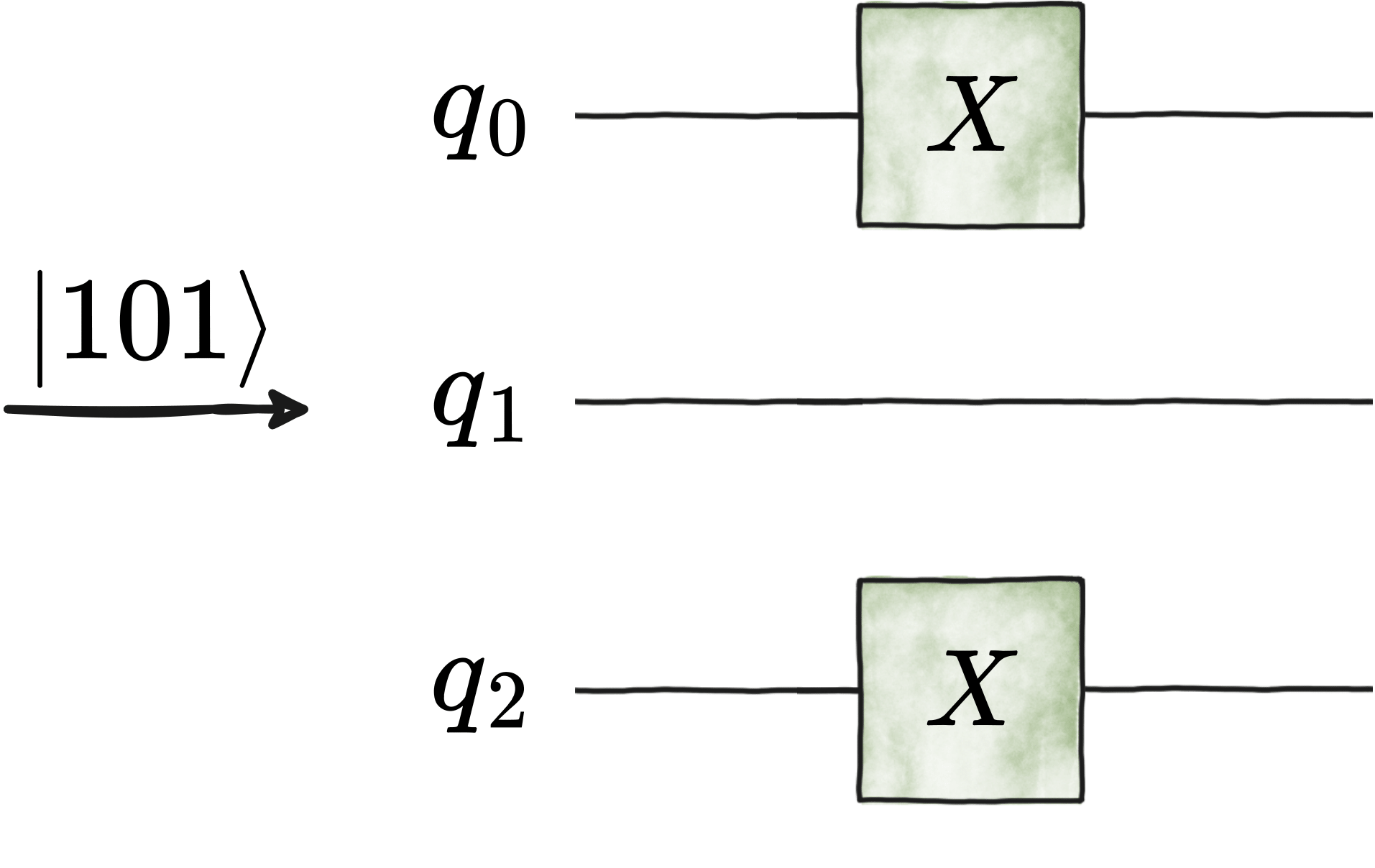
Given a bitstring $b$ of length $n$, this encoder generates a layer of Pauli-$X$ gates that creates the quantum state $|\,b\,\rangle$.

For instance, the following two circuit generations are equivalent:

b = "101"
circuit_1 = comp_basis_encoder(b)

circuit_2 = Circuit(3)
circuit_2.add(gates.X(0))
circuit_2.add(gates.X(2))

qibo.models.encodings.comp_basis_encoder(basis_element, nqubits=None, **kwargs)[source]#

Create circuit that performs encoding of bitstrings into computational basis states.

Parameters:

basis_element (int or str or list or tuple) – bitstring to be encoded. If int, nqubits must be specified. If str, must be composed of only $0`s and :math:`1`s. If ``list`$ or tuple, must be composed of $0`s and :math:`1`s as ``int`$ or str.
nqubits (int, optional) – total number of qubits in the circuit. If basis_element is int, nqubits must be specified. If nqubits is None, nqubits defaults to length of basis_element. Defaults to None.
kwargs (dict, optional) – Additional arguments used to initialize a Circuit object. For details, see the documentation of qibo.models.circuit.Circuit.

Returns:

Circuit encoding computational basis element.

Return type:

qibo.models.circuit.Circuit

Dicke state#

qibo.models.encodings.dicke_state(nqubits, weight, all_to_all=False, **kwargs)[source]#

Create a circuit that prepares the Dicke state $\ket{D_{k}^{n}}$.

The Dicke state $\ket{D_{k}^{n}}$ is the equal superposition of all $n$-qubit computational basis states with fixed-Hamming-weight $k$. The circuit prepares the state deterministically with $O(k \, n)$ gates and $O(n)$ depth, or $O(k \log\frac{n}{k})$ depth under the assumption of all-to-all connectivity.

Parameters:

nqubits (int) – number of qubits $n$.
weight (int) – Hamming weight $k$ of the Dicke state.
all_to_all (bool, optional) – If False, uses implementation from Ref. [1]. If True, uses shorter-depth implementation from Ref. [2]. Defaults to False.
kwargs (dict, optional) – additional arguments used to initialize a Circuit object. For details, see the documentation of qibo.models.circuit.Circuit.

Returns:

Circuit that prepares $\ket{D_{k}^{n}}$.

Return type:

qibo.models.circuit.Circuit

References

1. Andreas Bärtschi and Stephan Eidenbenz, Deterministic preparation of Dicke states, 22nd International Symposium on Fundamentals of Computation Theory, FCT’19, 126-139 (2019).

2. Andreas Bärtschi and Stephan Eidenbenz, Short-Depth Circuits for Dicke State Preparation, IEEE International Conference on Quantum Computing & Engineering (QCE), 87–96 (2022).

Entangling layer#

Generates a layer of nearest-neighbour two-qubit gates, assuming 1-dimensional connectivity. With the exception of qibo.gates.gates.GeneralizedfSim, any of the two-qubit gates implemented in qibo can be selected to customize the entangling layer. If the chosen gate is parametrized, all phases are set to $0.0$. Note that these phases can be updated a posterior by using qibo.models.Circuit.set_parameters(). The possible choices of layer architecture are the following, in alphabetical order: all-to-all, diagonal, even_layer, next_nearest, pyramid, odd_layer, shifted, v, and x. For instance, we show below an example of four of those architectures for nqubits = 6 and entangling_gate = "CNOT".

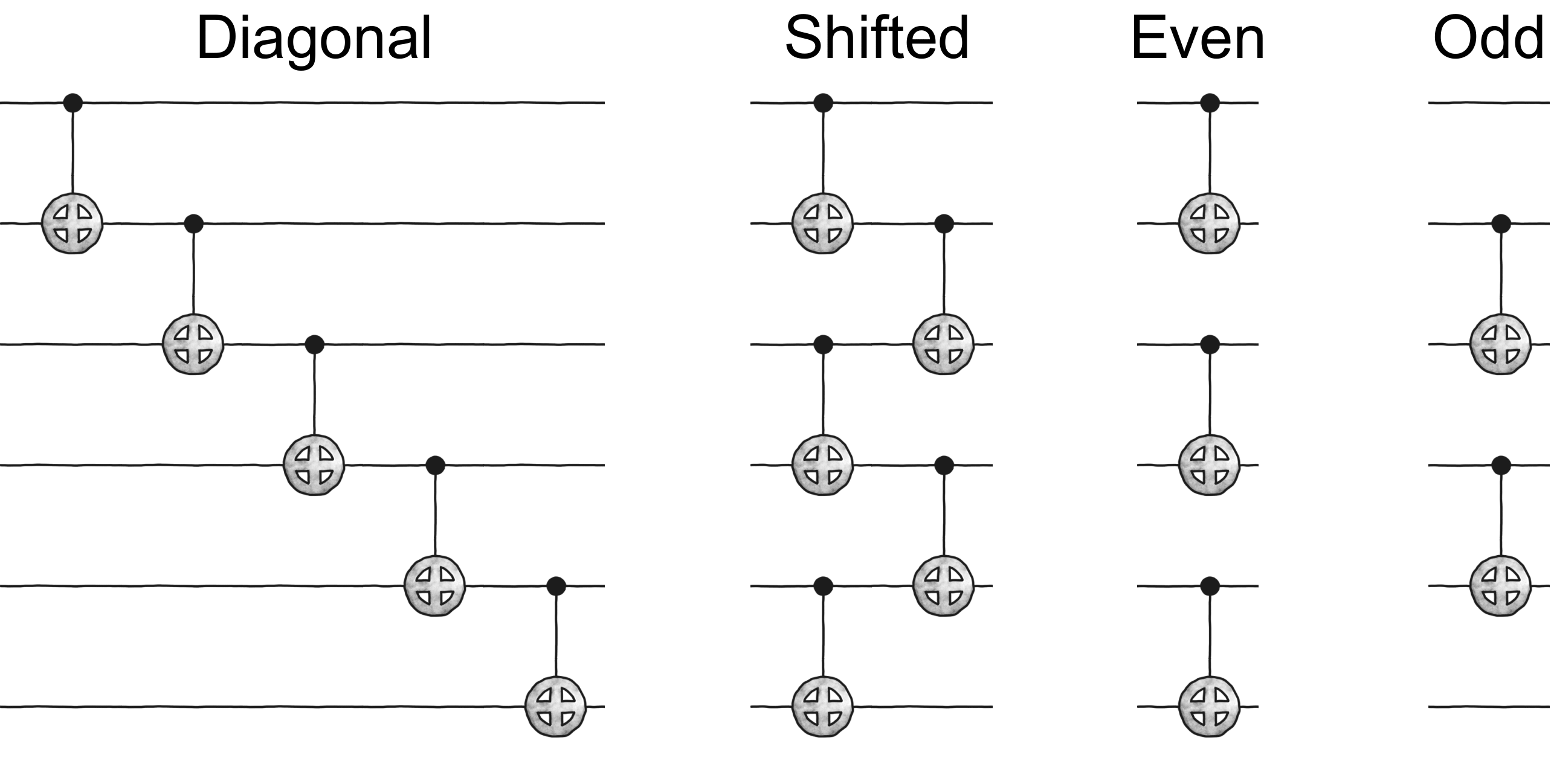
If closed_boundary is set to True, then an extra gate is added connecting the last and the first qubit, with the last qubit as the control qubit and the first qubit as a target qubit.

qibo.models.encodings.entangling_layer(nqubits, architecture='diagonal', entangling_gate='CNOT', closed_boundary=False, **kwargs)[source]#

Create a layer of two-qubit entangling gates.

If the chosen gate is a parametrized gate, all phases are set to $0.0$.

Parameters:

nqubits (int) – Total number of qubits in the circuit.
architecture (str, optional) – Architecture of the entangling layer. In alphabetical order, options are "all-to-all", "diagonal", "even_layer", "next_nearest", "odd_layer", "pyramid", "shifted", "v", and "x". The "all-to-all" architecture acts on all pairs of qubits $(j, k)$ with $j < k$, ordered such that the depth of the layer is minimal: $n - 1$ for even $n$ and $n$ for odd $n$. The "x" architecture is only defined for an even number of qubits. Defaults to "diagonal".
entangling_gate (str or qibo.gates.Gate, optional) – Two-qubit gate to be used in the entangling layer. If entangling_gate is a parametrized gate, all phases are initialized as $0.0$. Defaults to "CNOT".
closed_boundary (bool, optional) – If True and architecture not in ["all-to-all", "pyramid", "v", "x"], adds a closed-boundary condition to the entangling layer. Defaults to False.
kwargs (dict, optional) – Additional arguments used to initialize a Circuit object. For details, see the documentation of qibo.models.circuit.Circuit.

Returns:

Circuit containing layer of two-qubit gates.

Return type:

qibo.models.circuit.Circuit

Greenberger-Horne-Zeilinger (GHZ) state#

qibo.models.encodings.ghz_state(nqubits, **kwargs)[source]#

Generate an $n$-qubit Greenberger-Horne-Zeilinger (GHZ) state that takes the form

\[\ket{\text{GHZ}} = \frac{\ket{0}^{\otimes n} + \ket{1}^{\otimes n}}{\sqrt{2}}\]

where $n$ is the number of qubits.

Parameters:

nqubits (int) – number of qubits $n >= 2$.
kwargs (dict, optional) – additional arguments used to initialize a Circuit object. For details, see the documentation of qibo.models.circuit.Circuit.

Returns:

Circuit that prepares the GHZ state.

Return type:

qibo.models.circuit.Circuit

Graph state#

qibo.models.encodings.graph_state(matrix, backend=None, **kwargs)[source]#

Create circuit encoding an undirected graph state given its adjacency matrix.

Given a graph $G = (V, E)$ with $V$ being the set of vertices and $E$ being the set of edges, an $n$-qubit graph state is defined as

\[\ket{G} = \prod_{(j, k) \in E} \, CZ_{j, k} \, \ket{+}^{\otimes V} \, ,\]

where $CZ_{a,b}$ is the qibo.gates.CZ gate acting on qubits $j$ and $k$, and $\ket{+} = H \, \ket{0}$, with :class:`qibo.gates.H$ being the Hadamard gate.

Parameters:

matrix (ArrayLike or list) – Adjacency matrix of the graph.
backend (qibo.backends.abstract.Backend, optional) – backend to be used in the execution. If None, it uses the current backend. Defaults to None.
kwargs (dict, optional) – Additional arguments used to initialize a Circuit object. For details, see the documentation of qibo.models.circuit.Circuit.

Returns:

Circuit of the graph state with the given adjacency matrix.

Return type:

qibo.models.circuit.Circuit

Fanout gate synthesis in log depth#

qibo.models.encodings.fanout_synthesis(qubits, nqubits=None, method=None, **kwargs)[source]#

Synthesis of the Fanout gate in logarithmic depth.

Implementation based on applying Ref. [1, Algorithm 1] twice.

Parameters:

qubits (list[int] | tuple[int]) – qubits in which the CNOT ladder acts on.
nqubits (int, optional) – total number of qubits in the circuit. To be used when the total number of qubits differ from len(qubits). Defaults to None.
method (str, optional) – if “parity”, return a fanout decomposition based on parity trees. If None, return a decomposition based on CNOT-ladder synthesis. Defaults to None.

Returns:

Circuit containing the sequence of gates in parallel.

Return type:

qibo.models.circuit.Circuit

References

1. M. Remaud and V. Vanndaele, Ancilla-free quantum adder with sublinear depth, In: Glück, R., Kaarsgaard, R. (eds) Reversible Computation. RC 2025. Lecture Notes in Computer Science, vol 15716. Springer, Cham. (2025).

Fixed Hamming-weight Encoder#

qibo.models.encodings.hamming_weight_encoder(nqubits, weight, data=None, complex_data=False, full_hwp=False, optimize_controls=True, phase_correction=True, initial_string=None, backend=None, **kwargs)[source]#

Create circuit that encodes data in the Hamming-weight-$k$ basis of nqubits.

Let $\mathbf{x}$ be a $1$-dimensional array of size $d = \binom{n}{k}$ and $B_{k} \equiv \{ \ket{b_{j}} : b_{j} \in \{0, 1\}^{\otimes n} \,\, \text{and} \,\, |b_{j}| = k \}$ be a set of $d$ computational basis states of $n$ qubits that are represented by bitstrings of Hamming weight $k$. Then, an amplitude encoder in the basis $B_{k}$ is an $n$-qubit parameterized quantum circuit $\operatorname{Load}_{B_{k}}$ such that

\[\operatorname{Load}(\mathbf{x}) \, \ket{0}^{\otimes n} = \frac{1}{\|\mathbf{x}\|} \, \sum_{j = 1}^{d} \, x_{j} \, \ket{b_{j}}\]

Parameters:

nqubits (int) – number of qubits.
weight (int) – Hamming weight that defines the subspace in which data will be encoded.
data (ArrayLike, optional) – $1$-dimensional array of data to be loaded. If None, circuit is returned with all phases set to $0.0$. Defaults to None.
complex_data (bool, optional) – to be used when data is None. If True, returned circuit parametrizes complex-valued states. If False, it parametrizes real-valued states. If data is not None, then data type is inferred from data. Defaults to False.
full_hwp (bool, optional) – if False, includes Pauli-$X$ gates that prepare the first bitstring of Hamming weight k = weight. If True, circuit is full Hamming weight preserving. Defaults to `False.
optimize_controls (bool, optional) – if True, removes unnecessary controlled operations. Defaults to True.
phase_correction (bool, optional) – To be used when data is complex-valued. If True, adds a controlled-$mathrm{RZ}$ gate to the end of the circuit, adding a final phase correction. If False, gate is not added. Defaults to True.
initial_string (ArrayLike, optional) – Array containing the desired initial bitstring of Hamming weight $k$. If None, defaults to $ket{1^{k}0^{n-k}}$. Defaults to None.
backend (qibo.backends.abstract.Backend, optional) – backend to be used in the execution. If None, it uses the current backend. Defaults to None.
kwargs (dict, optional) – Additional arguments used to initialize a Circuit object. For details, see the documentation of qibo.models.circuit.Circuit.

Returns:

Circuit that loads data in Hamming-weight-$k$ representation.

Return type:

qibo.models.circuit.Circuit

References

1. R. M. S. Farias, T. O. Maciel, G. Camilo, R. Lin, S. Ramos-Calderer, and L. Aolita, Quantum encoder for fixed-Hamming-weight subspaces Phys. Rev. Applied 23, 044014 (2025).

CNOT ladder synthesis in log depth#

qibo.models.encodings.ladder_synthesis(qubits, nqubits=None, return_circuit=False, **kwargs)[source]#

Synthesis of the CNOT ladder operator in logarithmic depth.

Implementation based on Ref. [1, Algorithm 1].

Parameters:

qubits (list[int] | tuple[int]) – qubits in which the CNOT ladder acts on.
nqubits (int, optional) – total number of qubits in the circuit. To be used when return_circuit=True and the total number of qubits differ from len(qubits). Defaults to None.
return_circuit (bool, optional) – if True, returns a qibo.models.circuit.Circuit class. If False, returns a list with the sequence of qibo.gates.CNOT gates in parallel. Defaults to False.

Returns:

List of gates or circuit containing the sequence of gates.

Return type:

list or qibo.models.circuit.Circuit

References

Permutation synthesis#

qibo.models.encodings.permutation_synthesis(sigma, m=2, backend=None, **kwargs)[source]#

Return circuit that implements a given permutation.

Given permutation sigma on $\{0, \, 1, \, \dots, \, d-1\}$ and a power‑of‑two budget m, this function factors sigma into the fewest layers $\sigma_{1}, \, \sigma_{2}, \, \cdots, \, \sigma_{t}$ such that: - each layer has at most $m$ disjoint transpositions; - each layer moves a power‑of‑two number of indices.

The function returns a circuit synthesis of sigma.

Parameters:

sigma (list or tuple) – permutation description on $\{0, \, 1, \, \dots, \, d-1\}$.
m (int) – power‑of‑two budget. Defauls to $2$.
backend (qibo.backends.abstract.Backend, optional) – backend to be used in the execution. If None, it uses the current backend. Defaults to None.
kwargs (dict, optional) – Additional arguments used to initialize a Circuit object. For details, see the documentation of qibo.models.circuit.Circuit.

Returns:

Circuit that implements the permutation sigma.

Return type:

qibo.models.circuit.Circuit

References

1. L. Li, and J. Luo, Nearly Optimal Circuit Size for Sparse Quantum State Preparation arXiv:2406.16142 (2024).

Phase Encoder#

Encodes data of length $n$ into the phases of $n$ qubits.

For instance, the following two circuit generations are equivalent:

nqubits = 3
phases = np.random.rand(nqubits)

circuit_1 = phase_encoder(nqubits, rotation="RX", data=phases)

circuit_2 = Circuit(3)
circuit_2.add(gates.RX(qubit, phases[qubit]) for qubit in range(nqubits))

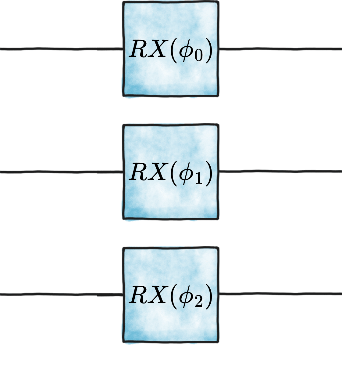
qibo.models.encodings.phase_encoder(nqubits, rotation='RY', data=None, backend=None, **kwargs)[source]#

Create circuit that performs the phase encoding of data.

Parameters:

nqubits (int) – number of qubits in the system.
rotation (str, optional) – If "RX", uses qibo.gates.gates.RX as rotation. If "RY", uses qibo.gates.gates.RY as rotation. If "RZ", uses qibo.gates.gates.RZ as rotation. Defaults to "RY".
data (ArrayLike) – $1$-dimensional array of phases to be loaded. If None, all phases of the circuit are set to $0.0$. Defaults to None.
backend (qibo.backends.abstract.Backend, optional) – backend to be used in the execution. If None, it uses the current backend. Defaults to None.
kwargs (dict, optional) – Additional arguments used to initialize a Circuit object. For details, see the documentation of qibo.models.circuit.Circuit.

Returns:

Circuit that loads data in phase encoding.

Return type:

qibo.models.circuit.Circuit

Sparse encoder#

qibo.models.encodings.sparse_encoder(data, method='li', nqubits=None, backend=None, **kwargs)[source]#

Create circuit that encodes $1$-dimensional data in a subset of amplitudes of the computational basis.

Consider a sparse-access model, where for a data vector $\mathbf{x} \in \mathbb{C}^{d}$, with $d = 2^{n}$ and $s$ non-zero amplitudes, one has access to the data vector $\mathbf{y}$ of the form

\[\mathbf{y} = \left\{ (b_{1}, x_{1}), \, \dots, \, (b_{s}, x_{s}) \right\} \, ,\]

where $\{x_{j}\}_{j\in[s]}$ is the non-zero components of $\mathbf{x}$ and $\{b_{j}\}_{j\in[s]}$ is the set of addresses associated with these values. Then, this function generates a quantum circuit $s\text{-}\mathrm{Load}$ that encodes $\mathbf{x}$ in the amplitudes of an $n$-qubit quantum state as

\[s\text{-}\mathrm{Load}(\mathbf{y}) \, \ket{0}^{\otimes \, n} = \sum_{j\in[s]} \, \frac{x_{j}}{\|\mathbf{x}\|_{2}} \, \ket{b_{j}} \, ,\]

where $\|\cdot\|_{2}$ is the Euclidean norm.

The resulting circuit parametrizes data in hyperspherical coordinates in the $(2^{n} - 1)$-unit sphere.

Parameters:

data (ArrayLike or list or zip) – sequence of tuples of the form $(b_{j}, x_{j})$. The addresses $b_{j}$ can be either integers or in bitstring format of size $n$.
method (str, optional) – method to be used, either li or farias. They refer to methods in references [1] and [2], respectively. Defaults to li
nqubits (int, optional) – total number of qubits in the system. To be used when $b_j$ are integers. If $b_j$ are strings and nqubits is None, defaults to the length of the strings $b_{j}$. Defaults to None.
backend (qibo.backends.abstract.Backend, optional) – backend to be used in the execution. If None, it uses the current backend. Defaults to None.
kwargs (dict, optional) – Additional arguments used to initialize a Circuit object. For details, see the documentation of qibo.models.circuit.Circuit.

Returns:

Circuit that loads sparse $\mathbf{x}$.

Return type:

qibo.models.circuit.Circuit

References

1. L. Li, and J. Luo, Nearly optimal circuit size for sparse quantum state preparation arXiv:2406.16142 (2024).

2. R. M. S. Farias, T. O. Maciel, G. Camilo, R. Lin, S. Ramos-Calderer, and L. Aolita, Quantum encoder for fixed-Hamming-weight subspaces, Phys. Rev. Applied 23, 044014 (2025).

Hyperpherical coordinates.

Spin-$s$ fixed-magnetization Encoder#

Generalization of the fixed Hamming-weight encoder to chains of $n$ spin-$s$ sites, loading data into the eigenspace of total magnetization $S^{z}$. Each site is mapped into qubits via either a unary or a binary encoding.

qibo.models.encodings.spin_s_encoder(nqudits, spin, weight, data=None, complex_data=False, encoding='unary', optimize_controls=True, phase_correction=True, backend=None, **kwargs)[source]#

Create circuit encoding data in a fixed-$S^{z}$ subspace of a spin-$s$ chain.

Let $\mathbf{x}$ be a $1$-dimensional array of size $D$ and $B_{k} \equiv \{ \ket{\mathbf{m}} : \mathbf{m} \in \{0, 1, \ldots, 2s\}^{n} \,\, \text{and} \,\, \sum_{r} m_{r} = k \}$ be the set of $D$ computational basis states of $n$ spin-$s$ sites (equivalently, $(2s + 1)$-level qudits) whose ditstrings $\mathbf{m}$ have fixed digit sum $k$. Then, this function returns a circuit $\operatorname{Load}_{B_{k}}$ such that

\[\operatorname{Load}(\mathbf{x}) \, \ket{0}^{\otimes n} = \frac{1}{\|\mathbf{x}\|} \, \sum_{j = 1}^{D} \, x_{j} \, \ket{\mathbf{m}_{j}} \, ,\]

where the ditstrings $\mathbf{m}_{j}$ are sorted in lexicographical order, with site $0$ being the most significant digit. The construction follows Refs. [1, 2]. For $s = 1/2$, this reduces to the fixed-Hamming-weight encoder of Ref. [3], implemented in qibo.models.encodings.hamming_weight_encoder().

Parameters:

nqudits (int) – number of spin-$s$ sites $n$.
spin (float) – spin $s \in \{1/2, \, 1, \, 3/2, \, \ldots\}$ of each site.
weight (int) – digit sum $k \in \{0, \, 1, \, \ldots, \, 2sn\}$ that defines the subspace in which data will be encoded.
data (ArrayLike, optional) – $1$-dimensional array of data to be loaded. If None, circuit is returned with all phases set to $0.0$. Defaults to None.
complex_data (bool, optional) – to be used when data is None. If True, returned circuit parametrizes complex-valued states. If False, it parametrizes real-valued states. If data is not None, then data type is inferred from data. Defaults to False.
encoding (str, optional) – mapping of each $(2s + 1)$-level site into qubits. Options are "unary" and "binary". Defaults to "unary".
optimize_controls (bool, optional) – if True, removes redundant controls on sites that were not modified by previous Gray gates, following Sec. 2.2.1 of Ref. [1]. Defaults to True.
phase_correction (bool, optional) – To be used when data is complex-valued. If True, adds a controlled-$\mathrm{RZ}$ gate to the end of the circuit, adding a final phase correction. If False, gate is not added. Defaults to True.
backend (qibo.backends.abstract.Backend, optional) – backend to be used in the execution. If None, it uses the current backend. Defaults to None.
kwargs (dict, optional) – Additional arguments used to initialize a Circuit object. For details, see the documentation of qibo.models.circuit.Circuit.

Returns:

Circuit that loads data in the fixed-digit-sum subspace of $n$ spin-$s$ sites.

Return type:

qibo.models.circuit.Circuit

References

1. N. Zare Harofteh and R. I. Nepomechie, Spin-s U(1)-eigenstate preparation, Ann. Phys. (Berlin) 538, e70239 (2026).

2. T. R. Walsh, Loop-free sequencing of bounded integer compositions, J. Comb. Math. Comb. Comp. 33, 323 (2000).

3. R. M. S. Farias, T. O. Maciel, G. Camilo, R. Lin, S. Ramos-Calderer, and L. Aolita, Quantum encoder for fixed-Hamming-weight subspaces Phys. Rev. Applied 23, 044014 (2025).

Unary Encoder#

Given a classical data array $\mathbf{x} \in \mathbb{R}^{d}$ such that

\[\mathbf{x} = (x_{1}, x_{2}, \dots, x_{d}) \, ,\]

this function generate the circuit that prepares the following quantum state $\ket{\psi} \in \mathcal{H}$:

\[\ket{\psi} = \frac{1}{\|\mathbf{x}\|_{\textup{HS}}} \, \sum_{k=1}^{d} \, x_{k} \, \ket{k} \, ,\]

with $\mathcal{H} \cong \mathbb{C}^{d}$ being a $d$-qubit Hilbert space, and $\|\cdot\|_{\textup{HS}}$ being the Hilbert-Schmidt norm.

Here, $\ket{k}$ is a unary representation of the number $k$. For instance, for $d = 3$, the final state would be

\[\ket{\psi} = \frac{1}{\|\mathbf{x}\|_{\textup{HS}}} \, \left( x_{1} \ket{001} + x_{2} \ket{010} + x_{3} \ket{100} \right) \, .\]

There are multiple circuit architechtures that lead to unary encoding of classical data. For example, to encode a $8$-dimensional data, one could use the so-called tree architechture below:

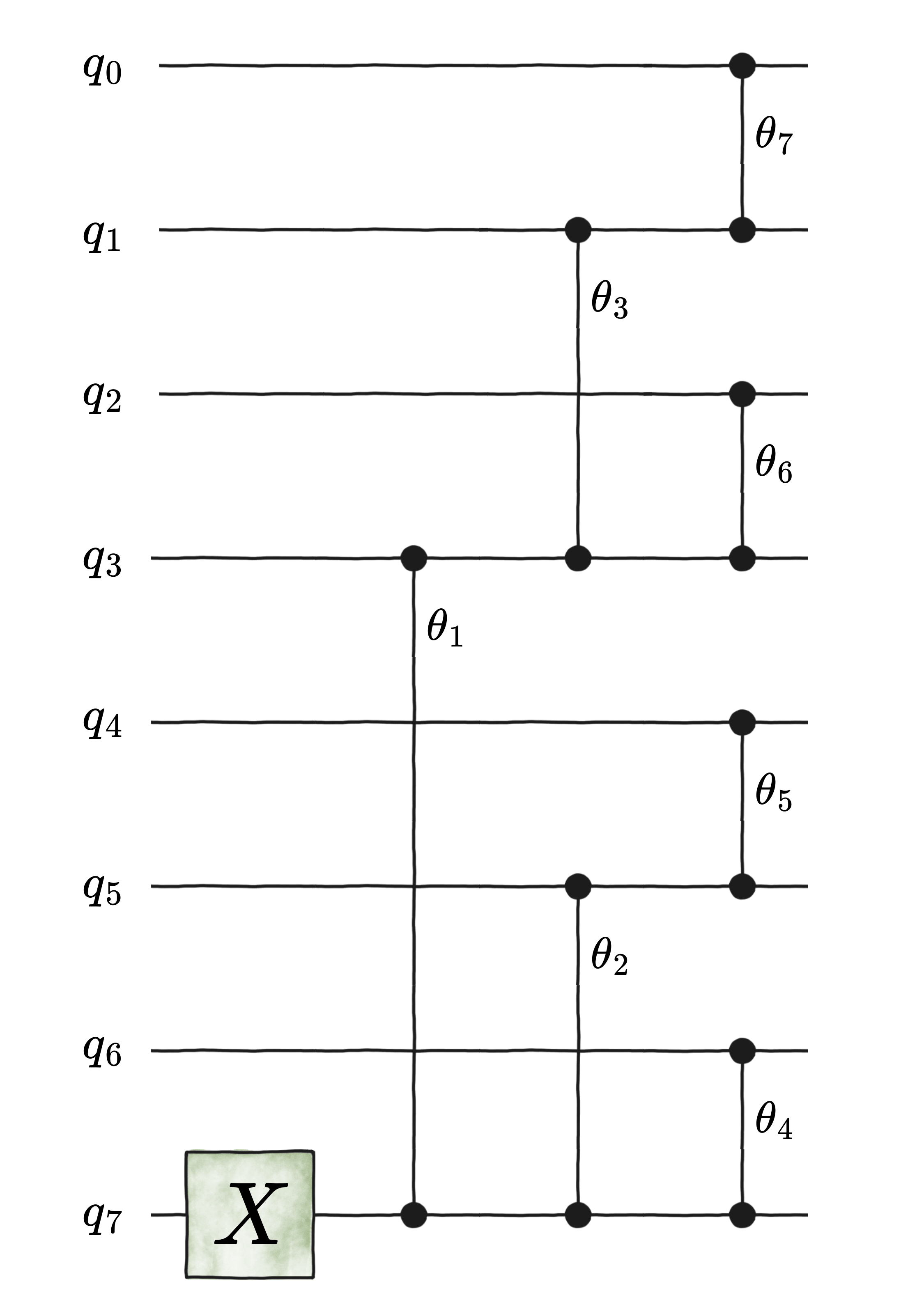
where the first gate is the qibo.gates.X and the parametrized gates are the qibo.gates.RBS. To know how the angles $\{\theta_{k}\}_{[k]}$ are calculated for this architecture, please refer to S. Johri et al., Nearest Centroid Classiﬁcation on a Trapped Ion Quantum Computer, arXiv:2012.04145v2 [quant-ph].

On the other hand, the same encoding could be performed using the so-called diagonal (also known as ladder) architecture below:

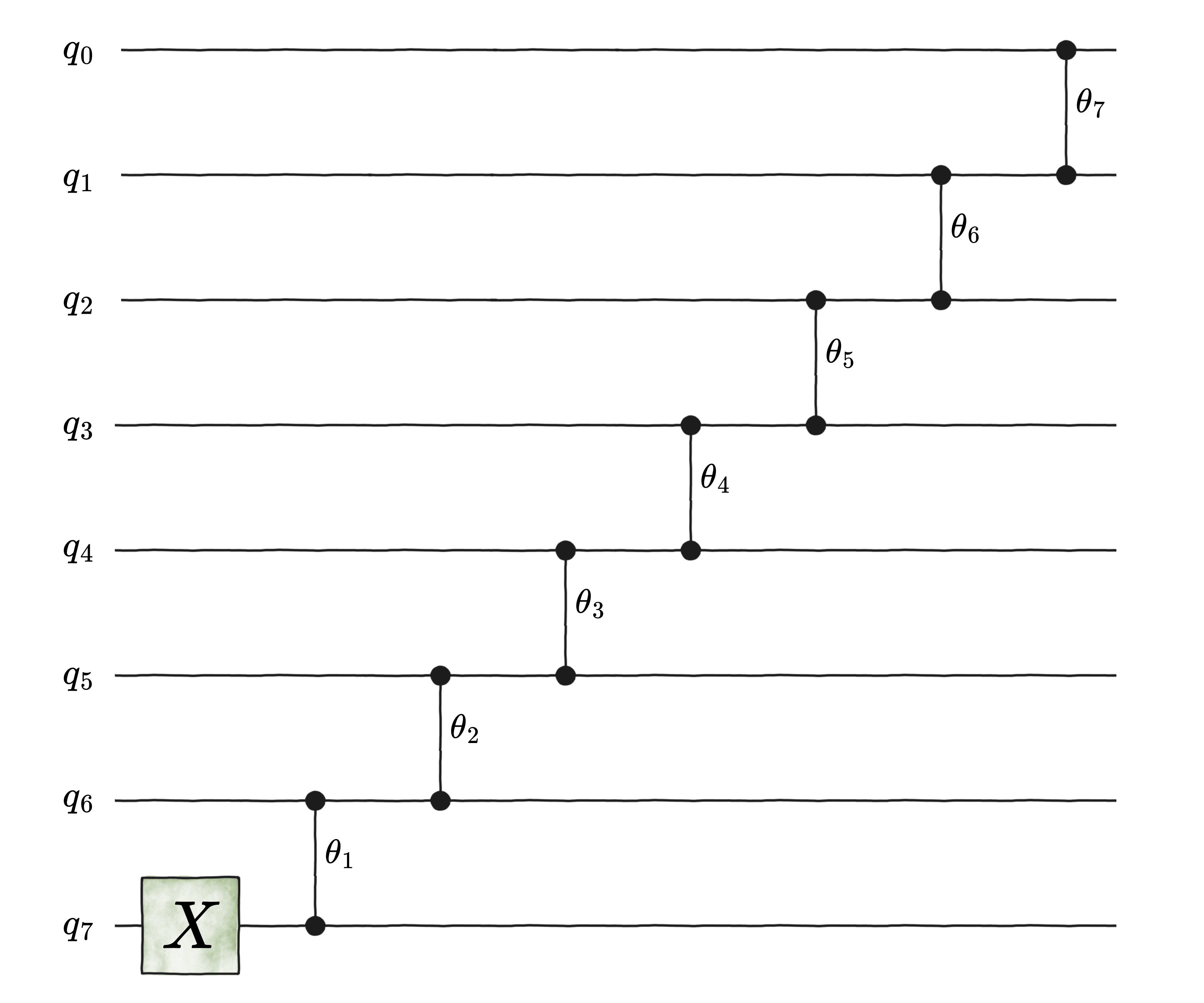
This architecture leads to a choice of angles based on spherical coordinates in a d-dimensional hypersphere.

qibo.models.encodings.unary_encoder(nqubits, architecture='tree', data=None, backend=None, **kwargs)[source]#

Create circuit that performs the (deterministic) unary encoding of data.

Parameters:

nqubits (int) – number of qubits in the system.
architecture (str, optional) – circuit architecture used for the unary loader. If diagonal, uses a ladder-like structure. If tree, uses a binary-tree-based structure. Defaults to tree.
data (ArrayLike) – $1$-dimensional array of data to be loaded. If None, all phases in the returned circuit are set to $0.0$.
backend (qibo.backends.abstract.Backend, optional) – backend to be used in the execution. If None, it uses the current backend. Defaults to None.
kwargs (dict, optional) – Additional arguments used to initialize a Circuit object. For details, see the documentation of qibo.models.circuit.Circuit.

Returns:

Circuit that loads data in unary representation.

Return type:

qibo.models.circuit.Circuit

Unary Encoder for Random Gaussian States#

Performs the same unary encoder as qibo.models.encodings.unary_encoder using the tree architecture , with the difference being that now each entry of the $d$-dimensional array is sampled from a Gaussian distribution $\mathcal{N}(0, 1)$.

qibo.models.encodings.unary_encoder_random_gaussian(nqubits, architecture='tree', seed=None, backend=None, **kwargs)[source]#

Create a circuit that performs the unary encoding of a random Gaussian state.

At depth $h$ of the tree architecture, the angles $\theta_{k} \in [0, 2\pi]$ of the the gates $RBS(\theta_{k})$ are sampled from the following probability density function:

\[p_{h}(\theta) = \frac{1}{2} \, \frac{\Gamma(2^{h-1})}{\Gamma^{2}(2^{h-2})} \, \left|\sin(\theta) \, \cos(\theta)\right|^{2^{h-1} - 1} \, ,\]

where $\Gamma(\cdot)$ is the Gamma function.

Parameters:

nqubits (int) – number of qubits.
architecture (str, optional) – circuit architecture used for the unary loader. If tree, uses a binary-tree-based structure. Defaults to tree.
seed (int or numpy.random.Generator, optional) – Either a generator of random numbers or a fixed seed to initialize a generator. If None, initializes a generator with a random seed. Defaults to None.
backend (qibo.backends.abstract.Backend, optional) – backend to be used in the execution. If None, it uses the current backend. Defaults to None.
kwargs (dict, optional) – Additional arguments used to initialize a Circuit object. For details, see the documentation of qibo.models.circuit.Circuit.

Returns:

Circuit that loads a random Gaussian array in unary representation.

Return type:

qibo.models.circuit.Circuit

References

1. A. Bouland, A. Dandapani, and A. Prakash, A quantum spectral method for simulating stochastic processes, with applications to Monte Carlo. arXiv:2303.06719v1 [quant-ph]

Up-to-Hamming-weight-$k$ Encoder#

qibo.models.encodings.up_to_k_hamming_weight_encoder(nqubits, up_to_k, data=None, complex_data=False, codewords=None, keep_antictrls=False, backend=None, **kwargs)[source]#

Create a circuit that encodes data in the Hamming-weight-$\leq k$ subspace of nqubits.

Let $\mathbf{x}$ be a $1$-dimensional array of size

\[d = \sum_{l=0}^{k} \binom{n}{l},\]

and define the union-Hamming-weight-subspace

\[B_{\le k} \equiv \left\{ \ket{b_j} : b_j \in \{0,1\}^{\otimes n}, \; |b_j| \le k \right\},\]

i.e., the set of all computational basis states of $n$ qubits whose bitstrings have Hamming weight less than or equal to $k$. Equivalently,

\[B_{\le k} = \bigcup_{w=0}^{k} B_w,\]

where $B_w$ denotes the set of basis states of fixed Hamming weight $w$.

An amplitude encoder in the basis $B_{\le k}$ is an $n$-qubit parameterized quantum circuit $\operatorname{Load}_{B_{\le k}}$ such that

\[\operatorname{Load}_{B_{\le k}}(\mathbf{x}) \, \ket{0}^{\otimes n} = \frac{1}{\|\mathbf{x}\|} \sum_{j=1}^{d} x_j \ket{b_j},\]

where $\{ \ket{b_j} \}_{j=1}^d$ is an enumeration of the elements of $B_{\le k}$.

Resulting circuit parametrizes data in either hyperspherical or hopf coordinates in the $(2^{n} - 1)$-unit sphere.

Parameters:

nqubits (int) – total number of qubits in the system.
up_to_k (int) – upper limit for the Hamming weight of the union-Hamming-weight-subspace in which the data to be loaded will be supported.
data (ArrayLike, optional) – $1$-dimensional array of length $d = \sum_{l=0}^{k} \binom{n}{l}$ to be loaded in the amplitudes of a $n$-qubit quantum state. If None, all phases of the returned circuit are set to $0.0$. Defaults to None.
complex_data (bool, optional) – to be used when data is None. If True, returned circuit parametrizes complex-valued states. If False, it parametrizes real-valued states. If data is not None, then data type is inferred from data. Defaults to False.
codewords (list, optional) – List of codewords used to encode the data in the given order. If None, the codewords are set by the erhlich algorithm.
keep_antictrls (bool, optional) – If True and parametrization is hyperspherical, we don’t simplify the anti-controls when placing the RBS gates. For details, see [1].
backend (qibo.backends.abstract.Backend, optional) – backend to be used in the execution. If None, it uses the current backend. Defaults to None.
kwargs (dict, optional) – Additional arguments used to initialize a Circuit object. For details, see the documentation of qibo.models.circuit.Circuit.

Returns:

Circuit that loads data in up-to-k encoding.

Return type:

qibo.models.circuit.Circuit

References

1. R. M. S. Farias, T. O. Maciel, G. Camilo, R. Lin, S. Ramos-Calderer, and L. Aolita, Quantum encoder for fixed-Hamming-weight subspaces Phys. Rev. Applied 23, 044014 (2025).

Hyperpherical coordinates.

Error Mitigation#

Qibo allows for mitigating noise in circuits via error mitigation methods. Unlike error correction, error mitigation does not aim to correct qubit errors, but rather it provides the means to estimate the noise-free expected value of an observable measured at the end of a noisy circuit.

Readout Mitigation#

A common kind of error happening in quantum circuits is readout error, i.e. the error in the measurement of the qubits at the end of the computation. In Qibo there are currently two methods implemented for mitigating readout errors, and both can be used as standalone functions or in combination with the other general mitigation methods by setting the paramter readout.

Response Matrix#

Given $n$ qubits, all the possible $2^n$ states are constructed via the application of the corresponding sequence of $X$ gates $X_0\otimes I_1\otimes\cdot\cdot\cdot\otimes X_{n-1}$. In the presence of readout errors, we will measure for each state $i$ some noisy frequencies $F_i^{noisy}$ different from the ideal ones $F_i^{ideal}=\delta_{i,j}$.

The effect of the error is modeled by the response matrix composed of the noisy frequencies as columns $M=\big(F_0^{noisy},...,F_{n-1}^{noisy}\big)$. We have indeed that:

\[F_i^{noisy} = M \cdot F_i^{ideal}\]

and, therefore, the calibration matrix obtained as $M_{\text{cal}}=M^{-1}$ can be used to recover the noise-free frequencies.

The calibration matrix $M_{\text{cal}}$ lacks stochasticity, resulting in a ‘negative probability’ issue. The distributions that arise after applying $M_{\text{cal}}$ are quasiprobabilities; the individual elements can be negative surpass 1, provided they sum to 1. It is posible to use Iterative Bayesian Unfolding (IBU) to preserve non-negativity. See Nachman et al for more details.

qibo.models.error_mitigation.get_response_matrix(nqubits, qubit_map=None, noise_model=None, nshots=10000, backend=None)[source]#

Computes the response matrix for readout mitigation.

Parameters:

nqubits (int) – Total number of qubits.
qubit_map (list, optional) – the qubit map. If None, a list of range of circuit’s qubits is used. Defaults to None.
noise_model (qibo.noise.NoiseModel, optional) – noise model used for simulating noisy computation. This matrix can be used to mitigate the effect of qibo.noise.ReadoutError.
nshots (int, optional) – number of shots. Defaults to $10000$.
backend (qibo.backends.abstract.Backend, optional) – backend to be used in the execution. If None, it uses the current backend. Defaults to None.

Returns:

the computed (nqubits, nqubits) response matrix for readout mitigation.

Return type:

ArrayLike

qibo.models.error_mitigation.iterative_bayesian_unfolding(probabilities, response_matrix, iterations=10)[source]#

Iterative Bayesian Unfolding (IBU) method for readout mitigation.

Parameters:

probabilities (ArrayLike) – the input probabilities to be unfolded.
response_matrix (ArrayLike) – the response matrix.
iterations (int, optional) – the number of iterations to perform. Defaults to 10.

Returns:

the unfolded probabilities.

Return type:

ArrayLike

Reference:: 1. B. Nachman, M. Urbanek et al, Unfolding Quantum Computer Readout Noise. arXiv:1910.01969 [quant-ph]. 2. S. Srinivasan, B. Pokharel et al, Scalable Measurement Error Mitigation via Iterative Bayesian Unfolding. arXiv:2210.12284 [quant-ph].

qibo.models.error_mitigation.apply_resp_mat_readout_mitigation(state, response_matrix, iterations=None)[source]#

Applies readout error mitigation to the given state using the provided response matrix.

Parameters:

state (qibo.measurements.CircuitResult) – the input state to be updated. This state should contain the frequencies that need to be mitigated.
response_matrix (numpy.ndarray) – the response matrix for readout mitigation.
iterations (int, optional) – the number of iterations to use for the Iterative Bayesian Unfolding method. If None the ‘inverse’ method is used. Defaults to None.

Returns:

the input state with the updated (mitigated) frequencies.

Return type:

qibo.measurements.CircuitResult

qibo.models.error_mitigation.apply_randomized_readout_mitigation(circuit, noise_model=None, nshots=10000, ncircuits=10, qubit_map=None, seed=None, backend=None)[source]#

Readout mitigation method that transforms the bias in an expectation value into a measurable multiplicative factor.

This factor can be eliminated at the expense of increased sampling complexity for the observable.

Parameters:

circuit (qibo.models.Circuit) – input circuit.
noise_model (qibo.noise.NoiseModel, optional) – noise model used for simulating noisy computation. Defaults to None.
nshots (int, optional) – number of shots. Defaults to $10000$.
ncircuits (int, optional) – number of randomized circuits. Each of them uses int(nshots / ncircuits) shots. Defaults to 10.
qubit_map (list, optional) – the qubit map. If None, a list of range of circuit’s qubits is used. Defaults to None.
seed (int or numpy.random.Generator, optional) – Either a generator of random numbers or a fixed seed to initialize a generator. If None, initializes a generator with a random seed. Default: None.
backend (qibo.backends.abstract.Backend, optional) – backend to be used in the execution. If None, it uses the current backend. Defaults to None.

Returns:

the state of the input circuit with: mitigated frequencies.

Return type:

qibo.measurements.CircuitResult

References

1. Ewout van den Berg, Zlatko K. Minev et al, Model-free readout-error mitigation for quantum expectation values. arXiv:2012.09738 [quant-ph].

qibo.models.error_mitigation.get_expectation_val_with_readout_mitigation(circuit, observable, noise_model=None, nshots=10000, readout=None, qubit_map=None, seed=None, backend=None)[source]#

CDR: Applies readout error mitigation to the given circuit and observable.

Parameters:

circuit (qibo.models.Circuit) – input circuit.
observable (qibo.hamiltonians.Hamiltonian/:class:`qibo.hamiltonians.SymbolicHamiltonian) – The observable to be measured.
noise_model (qibo.models.noise.NoiseModel, optional) – the noise model to be applied. Defaults to None.
nshots (int, optional) – the number of shots for the circuit execution. Defaults to $10^{4}$.
readout (dict, optional) –
a dictionary that may contain the following keys:
- ncircuits: int, specifies the number of random circuits to use for the randomized method of readout error mitigation.
- response_matrix: numpy.ndarray, used for applying a pre-computed response matrix for readout error mitigation.
- ibu_iters: int, specifies the number of iterations for the iterative Bayesian unfolding method of readout error mitigation. If provided, the corresponding readout error mitigation method is used. Defaults to an empty dict.
qubit_map (list, optional) – the qubit map. If None, a list of range of circuit’s qubits is used. Defaults to None.
seed (int or numpy.random.Generator, optional) – Either a generator of random numbers or a fixed seed to initialize a generator. If None, initializes a generator with a random seed. Default: None.
backend (qibo.backends.abstract.Backend, optional) – the backend to be used in the execution. If None, it uses the global backend. Defaults to None.

Returns:

The mitigated expectation value of the observable.

Return type:

float

Randomized readout mitigation#

This approach converts the effect of any noise map $A$ into a single multiplication factor for each Pauli observable, that is, diagonalizes the measurement channel. The multiplication factor $\lambda$ can be directly measured even without the quantum circuit. Dividing the measured value $\langle O\rangle_{noisy}$ by these factor results in the mitigated Pauli expectation value $\langle O\rangle_{ideal}$,

\[\langle O\rangle_{ideal} = \frac{\langle O\rangle_{noisy}}{\lambda}\]

This process can be implemented with the aforementioned qibo.models.error_mitigation.apply_randomized_readout_mitigation().

Zero Noise Extrapolation (ZNE)#

Given a noisy circuit $C$ and an observable $A$, Zero Noise Extrapolation (ZNE) consists in running $n+1$ versions of the circuit with different noise levels $\{c_j\}_{j=0..n}$ and, for each of them, measuring the expected value of the observable $E_j=\langle A\rangle_j$.

Then, an estimate for the expected value of the observable in the noise-free condition is obtained as:

\[\hat{E} = \sum_{j=0}^n \gamma_jE_j\]

with $\gamma_j$ satisfying:

\[\sum_{j=0}^n \gamma_j = 1 \qquad \sum_{j=0}^n \gamma_j c_j^k = 0 \quad \text{for}\,\, k=1,..,n\]

This implementation of ZNE relies on the insertion of gate pairs (that resolve to the identity in the noise-free case) to realize the different noise levels $\{c_j\}$, see He et al for more details. Hence, the canonical levels are mapped to the number of inserted pairs as $c_j\rightarrow 2 c_j + 1$.

qibo.models.error_mitigation.ZNE(circuit, observable, noise_levels, noise_model=None, nshots=10000, solve_for_gammas=False, global_unitary_folding=True, insertion_gate='CNOT', readout=None, qubit_map=None, seed=None, backend=None)[source]#

Runs the Zero Noise Extrapolation (ZNE) method for error mitigation.

The different noise levels are realized by the insertion of pairs of either CNOT or RX(pi/2) gates that resolve to the identiy in the noise-free case.

Parameters:

circuit (qibo.models.Circuit) – input circuit.
observable (qibo.hamiltonians.Hamiltonian or qibo.hamiltonians.SymbolicHamiltonian) – Observable to measure.
noise_levels (ndarray) – Sequence of noise levels.
noise_model (qibo.noise.NoiseModel, optional) – Noise model applied to simulate noisy computation.
nshots (int, optional) – Number of shots. Defaults to $10000$. If None, the circuit is simulated without sampling: with statevector simulation if noise_model is not None and with density matrix simulation otherwise. Readout mitigation is not available with exact simulation.
solve_for_gammas (bool, optional) – If True, explicitly solve the equations to obtain the gamma coefficients. Default is False.
global_unitary_folding (bool, optional) – If True, noise is increased by global unitary folding. If False, local unitary folding is used. Defaults to True.
insertion_gate (str, optional) – gate to be folded in the local unitary folding. If RX, the gate used is $RX(\pi / 2)$. Otherwise, it is the qibo.gates.gates.CNOT gate.
readout (dict, optional) –
a dictionary that may contain the following keys:
- ncircuits: int, specifies the number of random circuits to use for the randomized method of readout error mitigation.
- response_matrix: ndarray, used for applying a pre-computed response matrix for readout error mitigation.
- ibu_iters: int, specifies the number of iterations for the iterative Bayesian unfolding method of readout error mitigation. If provided, the corresponding readout error mitigation method is used. Defaults to an empty dict.
qubit_map (list, optional) – the qubit map. If None, a list of range of circuit’s qubits is used. Defaults to None.
seed (int or numpy.random.Generator, optional) – Either a generator of random numbers or a fixed seed to initialize a generator. If None, initializes a generator with a random seed. Default: None.
backend (qibo.backends.abstract.Backend, optional) – backend to be used in the execution. If None, it uses the current backend. Defaults to None.

Returns:

Estimate of the expected value of observable in the noise free condition.

Return type:

ArrayLike

Reference:: 1. K. Temme, S. Bravyi et al, Error mitigation for short-depth quantum circuits. Phys. Rev. Lett. 119, 180509 (2017).

qibo.models.error_mitigation.get_gammas(noise_levels, analytical=True)[source]#

Standalone function to compute the ZNE coefficients given the noise levels.

Parameters:

noise_levels (numpy.ndarray) – array containing the different noise levels. Note that in the CNOT insertion paradigm this corresponds to the number of CNOT pairs to be inserted. The canonical ZNE noise levels are obtained as 2 * c + 1.
analytical (bool, optional) – if True, computes the coeffients by solving the linear system. If False, use the analytical solution valid for the CNOT insertion method. Default is True.

Returns:

the computed coefficients.

Return type:

numpy.ndarray

qibo.models.error_mitigation.get_noisy_circuit(circuit, num_insertions, global_unitary_folding=True, insertion_gate=None)[source]#

Standalone function to generate the noisy circuit with the inverse gate pairs insertions.

Parameters:

circuit (qibo.models.circuit.Circuit) – circuit to modify.
num_insertions (int) – number of insertion gate pairs / global unitary folds to add.
global_unitary_folding (bool) – If True, noise is increased by global unitary folding. If False, local unitary folding is used. Defaults to True.
insertion_gate (str, optional) – gate to be folded in the local unitary folding. If RX, the gate used is $RX(\pi / 2)$. Otherwise, it is the CNOT gate.

Returns:

circuit with the inserted gate pairs or with global folding.

Return type:

qibo.models.Circuit

Clifford Data Regression (CDR)#

In the Clifford Data Regression (CDR) method, a set of $n$ circuits $S_n=\{C_i\}_{i=1,..,n}$ is generated starting from the original circuit $C_0$ by replacing some of the non-Clifford gates with Clifford ones. Given an observable $A$, all the circuits of $S_n$ are both simulated to obtain the correspondent expected values of $A$ in noise-free condition $\{a_i^{exact}\}_{i=1,..,n}$, and run in noisy conditions to obtain the noisy expected values $\{a_i^{noisy}\}_{i=1,..,n}$.

Finally a model $f$ is trained to minimize the mean squared error:

\[E = \sum_{i=1}^n \bigg(a_i^{exact}-f(a_i^{noisy})\bigg)^2\]

and learn the mapping $a^{noisy}\rightarrow a^{exact}$. The mitigated expected value of $A$ at the end of $C_0$ is then obtained simply with $f(a_0^{noisy})$.

In this implementation the initial circuit is expected to be decomposed in the three Clifford gates $RX(\frac{\pi}{2})$, $CNOT$, $X$ and in $RZ(\theta)$ (which is Clifford only for $\theta=\frac{n\pi}{2}$). By default the set of Clifford gates used for substitution is $\{RZ(0),RZ(\frac{\pi}{2}),RZ(\pi),RZ(\frac{3}{2}\pi)\}$. See Sopena et al for more details.

qibo.models.error_mitigation.CDR(circuit, observable, noise_model, nshots=10000, model=<function <lambda>>, n_training_samples=100, full_output=False, readout=None, qubit_map=None, seed=None, backend=None)[source]#

Runs the Clifford Data Regression error mitigation method.

Parameters:

circuit (qibo.models.Circuit) – input circuit decomposed in the primitive gates X, CNOT, RX(pi/2), RZ(theta).
observable (qibo.hamiltonians.Hamiltonian/:class:`qibo.hamiltonians.SymbolicHamiltonian) – observable to be measured.
noise_model (qibo.noise.NoiseModel) – noise model used for simulating noisy computation.
nshots (int, optional) – Number of shots. Defaults to $10000$. If None, the circuit is simulated without sampling: with statevector simulation if noise_model is not None and with density matrix simulation otherwise. Readout mitigation is not available with exact simulation.
model (callable, optional) – model used for fitting. This should be a callable function object f(x, *params), taking as input the predictor variable and the parameters. Default is a simple linear model f(x,a,b) := a*x + b.
n_training_samples (int, optional) – number of training circuits to sample. Defaults to $100$.
full_output (bool, optional) – if True, this function returns additional information: val, optimal_params, train_val. Defaults to False.
readout (dict, optional) –
a dictionary that may contain the following keys:
- ncircuits: int, specifies the number of random circuits to use for the randomized method of readout error mitigation.
- response_matrix: numpy.ndarray, used for applying a pre-computed response matrix for readout error mitigation.
- ibu_iters: int, specifies the number of iterations for the iterative Bayesian unfolding method of readout error mitigation. If provided, the corresponding readout error mitigation method is used. Defaults to an empty dict.
qubit_map (list, optional) – the qubit map. If None, a list of range of circuit’s qubits is used. Defaults to None.
seed (int or numpy.random.Generator, optional) – Either a generator of random numbers or a fixed seed to initialize a generator. If None, initializes a generator with a random seed. Default: None.
backend (qibo.backends.abstract.Backend, optional) – backend to be used in the execution. If None, it uses the current backend. Defaults to None.

Returns:

Mitigated expectation value of observable. val (float): Noisy expectation value of observable. optimal_params (list): Optimal values for params. train_val (dict): Contains the noise-free and noisy expectation values obtained with the training circuits.

Return type:

mit_val (float)

Reference:

P. Czarnik, A. Arrasmith et al, Error mitigation with Clifford quantum-circuit data. arXiv:2005.10189 [quant-ph].

qibo.models.error_mitigation.sample_training_circuit_cdr(circuit, replacement_gates=None, sigma=0.5, seed=None, backend=None)[source]#

Samples a training circuit for CDR by susbtituting some of the non-Clifford gates.

Parameters:

circuit (qibo.models.Circuit) – circuit to sample from, decomposed in RX(pi/2), X, CNOT and RZ gates.
replacement_gates (list, optional) – candidates for the substitution of the non-Clifford gates. The list should be composed by tuples of the form (gates.XYZ, kwargs). For example, phase gates are used by default: list((RZ, {'theta':0}), (RZ, {'theta':pi/2}), (RZ, {'theta':pi}), (RZ, {'theta':3*pi/2})).
sigma (float, optional) – standard devation of the Gaussian distribution used for sampling.
seed (int or numpy.random.Generator, optional) – Either a generator of random numbers or a fixed seed to initialize a generator. If None, initializes a generator with a random seed. Default: None.
backend (qibo.backends.abstract.Backend, optional) – backend to be used in the execution. If None, it uses the current backend. Defaults to None.

Returns:

The sampled circuit.

Return type:

qibo.models.Circuit

Variable Noise CDR (vnCDR)#

Variable Noise CDR (vnCDR) is an extension of the CDR method described above that factors in different noise levels as in ZNE. In detail, the set of circuits $S_n=\{\mathbf{C}_i\}_{i=1,..,n}$ is still generated as in CDR, but for each $\mathbf{C}_i$ we have $k$ different versions of it with increased noise $\mathbf{C}_i=C_i^0,C_i^1,...,C_i^{k-1}$.

Therefore, in this case we have a $k$-dimensional predictor variable $\mathbf{a}_i^{noisy}=\big(a_i^0, a_i^1,..,a_i^{k-1}\big)^{noisy}$ for the same noise-free targets $a_i^{exact}$, and we want to learn the mapping:

\[f:\mathbf{a}_i^{noisy}\rightarrow a_i^{exact}\]

via minimizing the same mean squared error:

\[E = \sum_{i=1}^n \bigg(a_i^{exact}-f(\mathbf{a}_i^{noisy})\bigg)^2\]

In particular, the default choice is to take $f(\mathbf{x}):=\Gamma\cdot \mathbf{x}\;$, with $\Gamma=\text{diag}(\gamma_0,\gamma_1,...,\gamma_{k-1})\;$, that corresponds to the ZNE calculation for the estimate of the expected value.

Here, as in the implementation of the CDR above, the circuit is supposed to be decomposed in the set of primitive gates ${RX(\frac{\pi}{2}),CNOT,X,RZ(\theta)}$. See Sopena et al for all the details.

qibo.models.error_mitigation.vnCDR(circuit, observable, noise_levels, noise_model, nshots=10000, model=None, n_training_samples=100, insertion_gate='CNOT', full_output=False, readout=None, qubit_map=None, seed=None, backend=None)[source]#

Runs the variable-noise Clifford Data Regression error mitigation method.

Parameters:

circuit (qibo.models.Circuit) – input circuit decomposed in the primitive gates X, CNOT, RX(pi/2), RZ(theta).
observable (qibo.hamiltonians.Hamiltonian or qibo.hamiltonians.SymbolicHamiltonian) – observable to be measured.
noise_levels (ArrayLike) – sequence of noise levels.
noise_model (qibo.noise.NoiseModel) – noise model used for simulating noisy computation.
nshots (int, optional) – Number of shots. Defaults to $10000$. If None, the circuit is simulated without sampling: with statevector simulation if noise_model is not None and with density matrix simulation otherwise. Readout mitigation is not available with exact simulation.
model (callable, optional) – model used for fitting. This should be a callable function object f(x, *params), taking as input the predictor variable and the parameters. Default is a simple linear model f(x,a,b) := a*x + b.
n_training_samples (int, optional) – number of training circuits to sample.
insertion_gate (str, optional) – gate to be used in the insertion. If "RX", the gate used is $RX(\pi / 2)$. Default is "CNOT".
full_output (bool, optional) – if True, this function returns additional information: val, optimal_params, train_val. Defaults to False.
readout (dict, optional) –
a dictionary that may contain the following keys:
- ncircuits: int, specifies the number of random circuits to use for the randomized method of readout error mitigation.
- response_matrix: numpy.ndarray, used for applying a pre-computed response matrix for readout error mitigation.
- ibu_iters: int, specifies the number of iterations for the iterative Bayesian unfolding method of readout error mitigation. If provided, the corresponding readout error mitigation method is used. Defaults to empty dict.
qubit_map (list, optional) – the qubit map. If None, a list of range of circuit’s qubits is used. Defaults to None.
seed (int or numpy.random.Generator, optional) – Either a generator of random numbers or a fixed seed to initialize a generator. If None, initializes a generator with a random seed. Default: None.
backend (qibo.backends.abstract.Backend, optional) – backend to be used in the execution. If None, it uses the current backend. Defaults to None.

Returns:

Mitigated expectation value of observable. val (list): Expectation value of observable with increased noise levels. optimal_params (list): Optimal values for params. train_val (dict): Contains the noise-free and noisy expectation values obtained with the training circuits.

Return type:

mit_val (float)

Reference:

A. Lowe, MH. Gordon et al, Unified approach to data-driven quantum error mitigation. arXiv:2011.01157 [quant-ph].

Importance Clifford Sampling (ICS)#

In the Importance Clifford Sampling (ICS) method, a set of $n$ circuits $S_n=\{C_i\}_{i=1,..,n}$ that stabilizes a given Pauli observable is generated starting from the original circuit $C_0$ by replacing all the non-Clifford gates with Clifford ones. Given an observable $A$, all the circuits of $S_n$ are both simulated to obtain the correspondent expected values of $A$ in noise-free condition $\{a_i^{exact}\}_{i=1,..,n}$, and run in noisy conditions to obtain the noisy expected values $\{a_i^{noisy}\}_{i=1,..,n}$.

Finally, a theoretically inspired model $f$ is learned using the training data.

The mitigated expected value of $A$ at the end of $C_0$ is then obtained simply with $f(a_0^{noisy})$.

qibo.models.error_mitigation.ICS(circuit, observable, readout=None, qubit_map=None, noise_model=None, nshots=10000, n_training_samples=10, full_output=False, seed=None, backend=None)[source]#

Computes the Important Clifford Sampling method.

Parameters:

circuit (qibo.models.Circuit) – input circuit.
observable (qibo.hamiltonians.Hamiltonian or qibo.hamiltonians.SymbolicHamiltonian) – the observable to be measured.
readout (dict, optional) –
a dictionary that may contain the following keys:
- ncircuits: int, specifies the number of random circuits to use for the randomized method of readout error mitigation.
- response_matrix: numpy.ndarray, used for applying a pre-computed response matrix for readout error mitigation.
- ibu_iters: int, specifies the number of iterations for the iterative Bayesian unfolding method of readout error mitigation. If provided, the corresponding readout error mitigation method is used. Defaults to an empty dict.
qubit_map (list, optional) – the qubit map. If None, a list of range of circuit’s qubits is used. Defaults to None.
noise_model (qibo.models.noise.NoiseModel, optional) – the noise model to be applied. Defaults to None.
nshots (int, optional) – Number of shots. Defaults to $10000$. If None, the circuit is simulated without sampling: with statevector simulation if noise_model is not None and with density matrix simulation otherwise. Readout mitigation is not available with exact simulation.
n_training_samples (int, optional) – the number of training samples. Defaults to 10.
full_output (bool, optional) – if True, this function returns additional information: val, optimal_params, train_val. Defaults to False.
seed (int or numpy.random.Generator, optional) – Either a generator of random numbers or a fixed seed to initialize a generator. If None, initializes a generator with a random seed. Default: None.
backend (qibo.backends.abstract.Backend, optional) – the backend to be used in the execution. If None, it uses the global backend. Defaults to None.

Returns:

the mitigated expectated value. mitigated_expectation_std (float): the standard deviation of the mitigated expectated value. dep_param (float): the depolarizing parameter. dep_param_std (float): the standard deviation of the depolarizing parameter. lambda_list (list): the list of the depolarizing parameters. data (dict): the data dictionary containing the noise-free and noisy expectation values obtained with the training circuits.

Return type:

mitigated_expectation (float)

Reference:: 1. Dayue Qin, Yanzhu Chen et al, Error statistics and scalability of quantum error mitigation formulas, npj Quantum Inf 9, 35 (2023).

qibo.models.error_mitigation.sample_clifford_training_circuit(circuit, seed=None, backend=None)[source]#

Samples a training circuit for CDR by susbtituting all the non-Clifford gates.

Parameters:

circuit (qibo.models.Circuit) – circuit to sample from.
seed (int or numpy.random.Generator, optional) – Either a generator of random numbers or a fixed seed to initialize a generator. If None, initializes a generator with a random seed. Default: None.
backend (qibo.backends.abstract.Backend, optional) – backend to be used in the execution. If None, it uses the current backend. Defaults to None.

Returns:

the sampled circuit.

Return type:

qibo.models.Circuit

Models#

Circuit models#

Circuit#

Circuit addition#

Circuit fusion#

Quantum Fourier Transform (QFT)#

Variational Quantum Eigensolver (VQE)#

Adiabatically Assisted Variational Quantum Eigensolver (AAVQE)#

Quantum Approximate Optimization Algorithm (QAOA)#

Feedback-based Algorithm for Quantum Optimization (FALQON)#

Grover’s Algorithm#

Double-Bracket Iterations#

Quantum Signal Processing#

Quantum Singular Value Transformation#

Block Encoding#

Linear Combination of Unitaries#

Iterative Quantum Amplitude Estimation (IQAE)#

Time evolution#

State evolution#

Adiabatic evolution#

Data Encoders#

Binary encoder#

Computational Basis Encoder#

Dicke state#

Entangling layer#

Greenberger-Horne-Zeilinger (GHZ) state#

Graph state#

Fanout gate synthesis in log depth#

Fixed Hamming-weight Encoder#

CNOT ladder synthesis in log depth#

Permutation synthesis#

Phase Encoder#

Sparse encoder#

Spin-\(s\) fixed-magnetization Encoder#

Unary Encoder#

Unary Encoder for Random Gaussian States#

Up-to-Hamming-weight-\(k\) Encoder#

Error Mitigation#

Readout Mitigation#

Response Matrix#

Randomized readout mitigation#

Zero Noise Extrapolation (ZNE)#

Clifford Data Regression (CDR)#

Variable Noise CDR (vnCDR)#

Importance Clifford Sampling (ICS)#