Quantum unary approach to option pricing#
Code at: https://github.com/qiboteam/qibo/tree/master/examples/unary
Based in the paper arXiv:1912.01618. In this README.md file you can see a short
set of instructions for the usage of the example.
What this example does?#
This example provides a new strategy to compute the expected payoff of a given (European) option using quantum computing. It is based on three previous results:
the Black-Scholes model, a classical model that models the behavior of an asset in the market
Amplitude Estimation, a quantum procedure to estimate the probability of obtaining some outcomes from a quantum circuit, providing quantum advantage
option pricing in quantum computers, a previous paper arXiv:1905.02666
The main feature of this procedure is to use the unary encoding of prices, that is, we work in the subspace of the Hilbert space where only one qubit is in the |1> state. This allows for a simplification of the circuit and resilience against errors, what makes the algorithm more suitable for NISQ devices. In contradistinction, it has an exponential overhead in the number of qubits as compared to the standard approaches. That makes our algorithm more efficient only when the problem is not very large.
The algorithm is divided in three steps. First, the probability distribution as computed in the Black-Scholes model is loaded into the quantum circuit by means of an exact circuit using iSWAP gates. Then, the payoff is computed by applying some controlled rotations on an ancilla qubit. Amplitude Estimation can be applied if the algorithm is applied and reversed together with some extra operations to achieve quantum advantage.
Usage#
In this example there are only three files
aux_functions.pycontains the classical functions that are needed to run the experiment.functions.pyencodes all quantum circuits and procedures needed to run the circuits.main.pyis the file calling all other functions. The action of every line of code is commented in the source code.
The parameters to be fixed for a run of the experiment are
S0: initial price of the assetK: strike of the European optionsig: volatility of the assetr: interest rate of the assetT: maturity dateshots: number of times the quantum experiments are ranbins: number of bins (qubits) used for the experimentmax_m: number of applications of the Q operator in Amplitude Estimation for the last step, increasing linearly (see the original paper for more details)
Results#
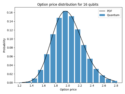
Three different results are presented in this example. First, it is shown how the amplitude distributor fits the predictions of the Black-Scholes model. As more qubits are added to the simulation, the approximation gets closer to the classical prediction.

The second result is printed in the console after every run of the example. It returns the exact classical value of the expected payoff, the expected payoff returned in the quantum experiment and the percentage error.
Exact value of the expected payoff:      0.15950474339651186

Expected payoff from quantum simulation: 0.16071698625159084

Percentage error: 0.7600042664972508 %
Finally, results in amplitude estimation are provided.
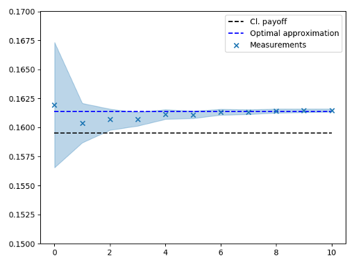
First, it is clear to see how the expected results converge to the optimal quantum result. Notice that the optimal quantum result is not exactly the exact classical value. This is due to discretization errors.

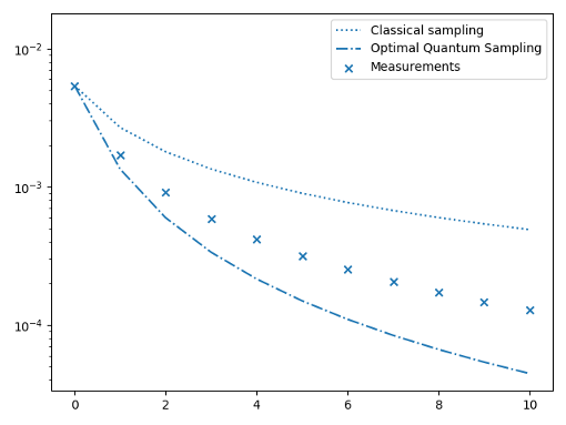
Second, it is worthy to study how the uncertainties in the outcomes evolve with the number of Amplitude Estimation iterations. Here it is depicted how these uncertainties are always lower than the classical standard Monte Carlo ones, but larger than the optimal quantum uncertainties. The reason is that the depth of the circuit is controlled to increase linearly, in order to control de errors in the circuit.

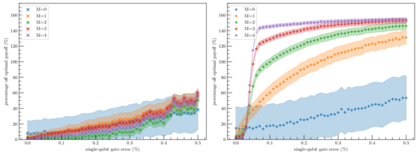
The ultimate strength of this algorithm is its resilience to errors in the circuit. The figure below describes the errors obtained for our algorithm (left) as compared to the method proposed in arXiv:1905.02666 (right) when noise is considered for 8 bins.
