Simple Adiabatic Evolution Examples#
Code at: https://github.com/qiboteam/qibo/tree/master/examples/adiabatic
Introduction#
Qibo provides models for simulating the unitary evolution of state vectors as well adiabatic evolution. The goal of adiabatic evolution is to find the ground state of a “hard” Hamiltonian H1. To do so, an “easy” Hamiltonian H0 is selected and the system is prepared in its ground state. The system is then left to evolve under the slowly changing Hamiltonian H(t) = (1 - s(t)) H0 + s(t) H1 for a total time T. If the scheduling function s(t) and the total time T are chosen appropriately the state at the end of this evolution will be the ground state of H1.
This example contains two scripts. The first performs the adiabatic evolution for a given choice of s(t) and T and plots the dynamics of the H1 energy as well as the overlap between the evolved state and the actual ground state of H1, which can be calculated via exact diagonalization for small systems. The second script optimizes the total time T and a parametrized family of s(t). Both scripts a sum of X operators H0 and the transverse field Ising model as H1.
Adiabatic evolution dynamics#
A simple adiabatic evolution example can be run using the linear.py script.
This supports the following options:
nqubits(int): Number of qubits in the system.hfield(float): Transverse field Ising model (qibo.hamiltonians.TFIM) h-field h value.T(int): Total time of the adiabatic evolution.dt(float): Time step used for integration.solver(str): Solver used for integration.
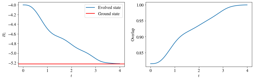
The following plots correspond to the adiabatic evolution of N=4 qubits for total time T=4 using linear scaling s(t)=t/T. At the left we show how the expectation value of H1 changes during evolution and at the right we plot the overlap between the evolved state and the ground state of H1. We see that at the end of evolution the evolved state reaches the ground state.
To gain more insight on the importance of the total evolution time T, we repeat the evolution for various choices of T and check how it affects the final energy and overlap. This is shown in the following plot
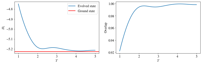
We see that the best overlap for this example is obtained for T=4.
Optimizing scheduling#
An example of scheduling function optimization can be run using the optimize.py
script. This optimizes a polynomial ansatz for s(t) using the H1
energy as the loss function. The total evolution time T is also optimized as an
additional free parameter. The following options are supported:
nqubits(int): Number of qubits in the system.hfield(float): Transverse field Ising model (qibo.hamiltonians.TFIM) h-field h value.params(str): Initial guess for free parameters. The numbers should be seperated using,. The last parameter is the initial guess for the total time T. The rest parameters are used to define the polynomial for s(t).dt(float): Time step used for integration.solver(str): Solver used for integration.method(str): Which scipy optimizer to use.maxiter(int): Maximum iterations for scipy optimizer.save(str): Name to use for saving optimization history. IfNonehistory will not be saved.
The following plots correspond to the optimization of a 3rd order polynomial for s(t). The first plot shows the final form of s(t) after optimization. The second plot shows how the loss function changes during optimization. The second line of plots shows the dynamics of the H1 energy and the overlap with the actual ground state when using the optimized schedule s(t) and total time T.
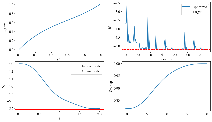
Note that the optimized 3rd order polynomial s(t) is capable of reaching a good approximation of the ground state energy after total time T=2 which is less than the T=4 required for the linear s(t) analyzed in the previous section.
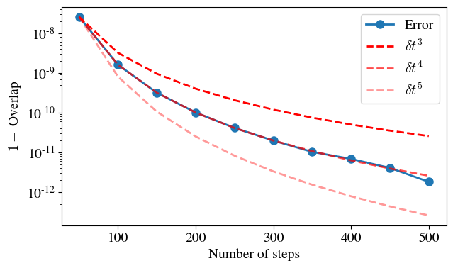
Error of Trotter decomposition#
The trotter_error.py script can be used to analyze the errors of time
evolution that uses the Trotter decomposition. The overlap between the final
state obtained using Trotter operators and the exact final state is used to
quantify this error. The script uses the transverse field Ising model as the
evolution Hamiltonian and supports the following options:
nqubits(int): Number of qubits in the system.hfield(float): Transverse field Ising model h-field h value.T(float): Total time of the adiabatic evolution.save(bool): Whether to save the plots.
In the following plot we see that for N=6 qubits, the error as quantified by 1 - overlap scales as dt^4.