Quantum Fourier Iterative Amplitude Estimation#
Code at: https://github.com/qiboteam/qibo/tree/master/examples/qfiae.
Based on the paper arXiv:2305.01686
Problem overview#
This tutorial implements an example of the application of the Quantum Fourier Iterative Amplitude Estimation (QFIAE) method, which allows to perform Quantum Monte Carlo integration of any one-dimensional function \(f(x)\).
The QFIAE algorithm functioning is the following:
The function we want to integrate \(f(x)\), the probability distribution \(p(x)\) and the limits of the integral \(x_{min}\), \(x_{max}\) are defined
A Quantum Neural Network (QNN) is employed to fit the function \(f(x)\) using a linear ansatz of the following form:
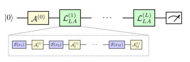
where \(\mathcal{L}^{(i)}\) is the i-th layer, that for the one-dimensional case is composed of the trainable gates:
and the encoding gate:
Now, as demonstrated in arXiv:2008.08605 the expectation value of this quantum model corresponds to a universal 1-D Fourier series:
The Fourier coefficients of the quantum circuit that fits the function \(f(x)\) are extracted using discrete Fourier transform
The Iterative Quantum Amplitude Estimation (IQAE) model of qibo, which corresponds with the following quantum circuit:
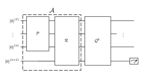
is used to estimate the integral of each trigonometric piece, \(\sin(\omega_i x)\) or \(\cos(\omega_j x)\), of the Fourier series.
The integrals obtained are summed with their corresponding coefficients to derive the final integral result.
A summary of the workflow of the algorithm is the following: 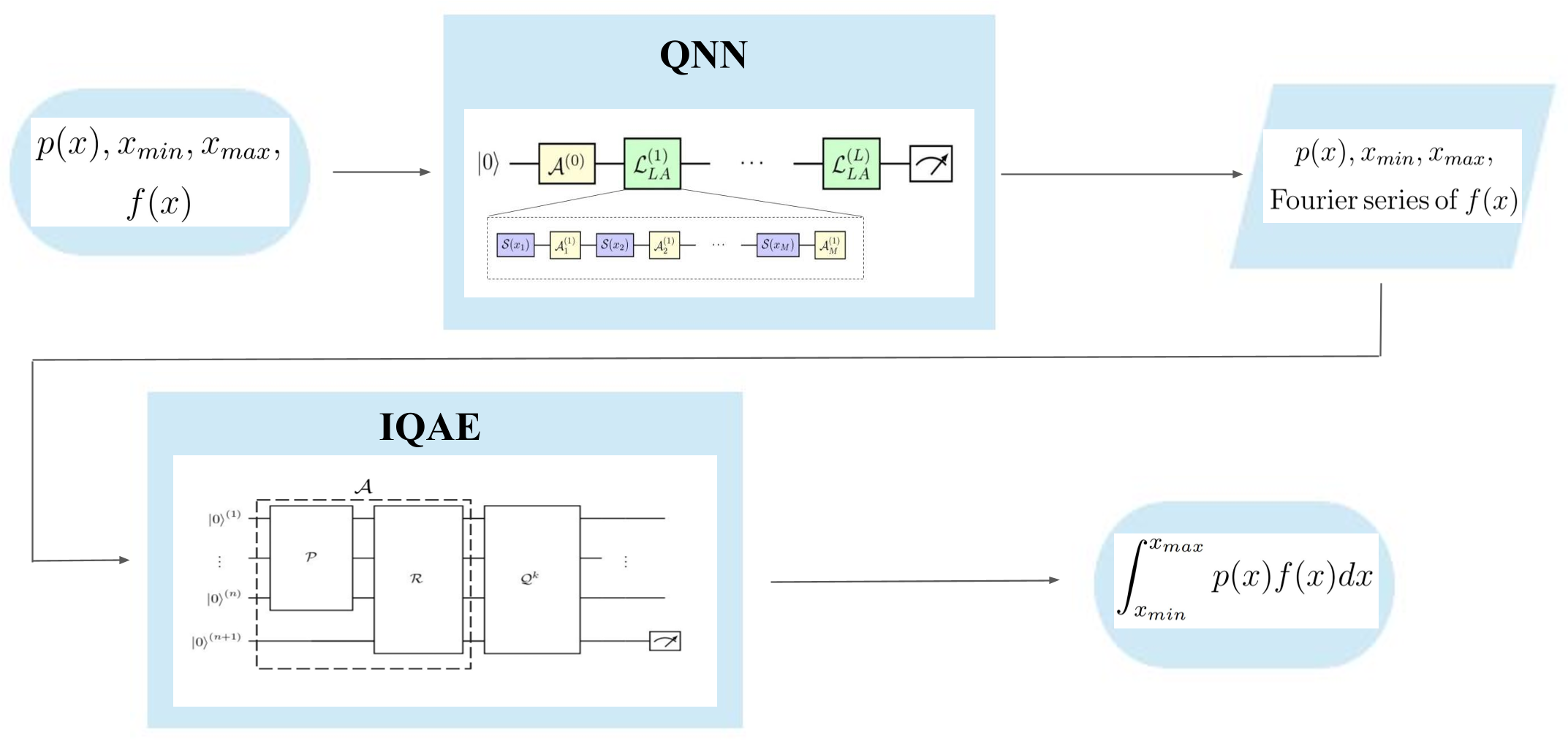
QFIAE Demo#
Let’s define the problem:
We are interested in computing the following example integral:
so the easiest way to define our problem variables would be:
\(x_{min}\): \(0\)
\(x_{max}\): \(1\)
\(p(x)\): \(dx\)
\(f(x)\): \(1+x^2\)
Code#
First, we must decide the variables for our problem.
Regarding the definition of the problem:
x_min_int: the lower limit of the problem integral.x_max_int: the upper limit of the problem integral.
Regarding the QNN:
nlayers: number of layers of the QNN.nepochs: number of epochs, i.e. iterations of the AdamDescent Optimizer.loss_treshold: value of the desired loss function’s treshold.learning_rate: learning rate of the AdamDescent Optimizer.nbatches: number of batches in which divide the dataset.ndata_points: number of data points to define \(f(x)\).x_max_fit: upper limit of the function we are going to fit.x_min_fit: lower limit of the function we are going to fit.
Regarding the IQAE:
nqubits: number of qubits decided to build the good state in the IQAE algorithm.alpha: confidence level, the target probability is 1 -alpha, has values between 0 and 1.epsilon: target precision for estimation target \(a\), has values between 0 and 0.5.nshots: number of shots used to perform IQAE.method_iqae: statistical method employed by IQAE. It will be chernoff or beta.
Regardind the results:
qfiae_integral: estimated value of the integral using QFIAE.iae_error: statistical uncertainty in the integral estimation due to IQAE.
Include necessary packages:
[1]:
import numpy as np

from qibo import Circuit, gates
from qibo.models.iqae import IQAE
1. Defining \(f(x)\), \(x_{min}\), \(x_{max}\)#
[2]:
def f(x):
    """Target function f(x) = 1 + x ^ 2"""

    y = 1 + x ** 2
    return y

x_min_int = 0
x_max_int = 1
2. Defining and training the QNN#
We import the QNN: vqregressor_linear_ansatz, which is a modified version of the vqregressor found at https://github.com/qiboteam/qibo/tree/master/examples/vqregressor. In our modified version, we replace the ansatz function used in the original implementation with the one we have previously defined.
[3]:
from vqregressor_linear_ansatz import VQRegressor_linear_ansatz
We define the parameters of the QNN
[4]:
# Note that the chosen number of layers is intentionally larger than necessary to fit the function.
# This configuration ensures high accuracy while keeping a reasonable number of epochs.
nlayers = 10
nepochs = 100
loss_treshold = 10^-4
learning_rate = 0.05
nbatches = 1
ndata_points = 200
# Note they can be different than x_min,x_max, but [x_max,x_min] ⊆ [x_max_fit,x_min_fit]
x_max_fit = 1
x_min_fit = -1
[5]:
np.random.seed(27)
vqr = VQRegressor_linear_ansatz(layers=nlayers,
ndata=ndata_points,
function=f, xmax=x_max_fit,
xmin=x_min_fit)
# With the selected configuration, the training usually takes around 30'
vqr.train_with_psr(
epochs=nepochs,
learning_rate=learning_rate,
batches=nbatches,
J_treshold=loss_treshold,
)
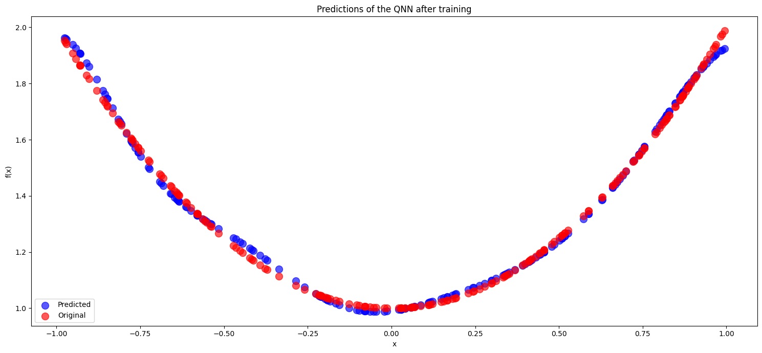
vqr.show_predictions("Predictions of the QNN after training", False)
[Qibo 0.1.16|INFO|2023-07-31 08:50:42]: Using qibojit (numba) backend on /CPU:0
Iteration  1  epoch  1  | loss:  0.7513285431118756
Iteration  2  epoch  2  | loss:  0.49078195900193
Iteration  3  epoch  3  | loss:  0.25449817735514246
Iteration  4  epoch  4  | loss:  0.1246609331106105
Iteration  5  epoch  5  | loss:  0.0656780490580047
Iteration  6  epoch  6  | loss:  0.033157170041590786
Iteration  7  epoch  7  | loss:  0.021080634318318345
Iteration  8  epoch  8  | loss:  0.02302933284076279
Iteration  9  epoch  9  | loss:  0.02804566383739096
Iteration  10  epoch  10  | loss:  0.02993298809989462
Iteration  11  epoch  11  | loss:  0.02809272996633005
Iteration  12  epoch  12  | loss:  0.024260018563301875
Iteration  13  epoch  13  | loss:  0.020466737677239978
Iteration  14  epoch  14  | loss:  0.017961154451515637
Iteration  15  epoch  15  | loss:  0.01635525503721851
Iteration  16  epoch  16  | loss:  0.013824870329752614
Iteration  17  epoch  17  | loss:  0.009480363571353416
Iteration  18  epoch  18  | loss:  0.005428317914456559
Iteration  19  epoch  19  | loss:  0.004747379983842302
Iteration  20  epoch  20  | loss:  0.007261736229780217
Iteration  21  epoch  21  | loss:  0.008972805823541971
Iteration  22  epoch  22  | loss:  0.006995705828705413
Iteration  23  epoch  23  | loss:  0.0031234835775331904
Iteration  24  epoch  24  | loss:  0.0010645149525778657
Iteration  25  epoch  25  | loss:  0.001660608449799947
Iteration  26  epoch  26  | loss:  0.0024468184819136764
Iteration  27  epoch  27  | loss:  0.0019337945857293712
Iteration  28  epoch  28  | loss:  0.0012357754610404163
Iteration  29  epoch  29  | loss:  0.0013015455646036862
Iteration  30  epoch  30  | loss:  0.0016682446926897167
Iteration  31  epoch  31  | loss:  0.0016495496176469587
Iteration  32  epoch  32  | loss:  0.0012520977035885572
Iteration  33  epoch  33  | loss:  0.0009722650541584987
Iteration  34  epoch  34  | loss:  0.0010738639185073821
Iteration  35  epoch  35  | loss:  0.001237623835436679
Iteration  36  epoch  36  | loss:  0.001079914927835038
Iteration  37  epoch  37  | loss:  0.0008087925855009583
Iteration  38  epoch  38  | loss:  0.0008412140573143836
Iteration  39  epoch  39  | loss:  0.0010243360494146807
Iteration  40  epoch  40  | loss:  0.0009260517614442422
Iteration  41  epoch  41  | loss:  0.0006083674444202678
Iteration  42  epoch  42  | loss:  0.00048552087540479593
Iteration  43  epoch  43  | loss:  0.0006110987021632932
Iteration  44  epoch  44  | loss:  0.0006559683517174265
Iteration  45  epoch  45  | loss:  0.0005150053878726019
Iteration  46  epoch  46  | loss:  0.0004114721142009153
Iteration  47  epoch  47  | loss:  0.0004471177670137205
Iteration  48  epoch  48  | loss:  0.0004770075457458069
Iteration  49  epoch  49  | loss:  0.00040857499834427296
Iteration  50  epoch  50  | loss:  0.00033020904524591827
Iteration  51  epoch  51  | loss:  0.0003179087176282798
Iteration  52  epoch  52  | loss:  0.00032425348191094495
Iteration  53  epoch  53  | loss:  0.0003081269055732997
Iteration  54  epoch  54  | loss:  0.00029739364175727137
Iteration  55  epoch  55  | loss:  0.0002972067254557964
Iteration  56  epoch  56  | loss:  0.0002790839752707141
Iteration  57  epoch  57  | loss:  0.000250994009314296
Iteration  58  epoch  58  | loss:  0.00024068099758678817
Iteration  59  epoch  59  | loss:  0.00024012049242896222
Iteration  60  epoch  60  | loss:  0.00023072309010057932
Iteration  61  epoch  61  | loss:  0.0002204255806400206
Iteration  62  epoch  62  | loss:  0.00021693211012467254
Iteration  63  epoch  63  | loss:  0.00021032053408251615
Iteration  64  epoch  64  | loss:  0.00019814302410227347
Iteration  65  epoch  65  | loss:  0.00018970104609909337
Iteration  66  epoch  66  | loss:  0.0001849409887409433
Iteration  67  epoch  67  | loss:  0.000178175085771177
Iteration  68  epoch  68  | loss:  0.00017235266528996997
Iteration  69  epoch  69  | loss:  0.00016920670127216307
Iteration  70  epoch  70  | loss:  0.00016352665275946328
Iteration  71  epoch  71  | loss:  0.0001558330982688153
Iteration  72  epoch  72  | loss:  0.00015122871287318634
Iteration  73  epoch  73  | loss:  0.0001481650541488665
Iteration  74  epoch  74  | loss:  0.0001435783238101642
Iteration  75  epoch  75  | loss:  0.000139808928386417
Iteration  76  epoch  76  | loss:  0.00013763074842478883
Iteration  77  epoch  77  | loss:  0.00013405673992693997
Iteration  78  epoch  78  | loss:  0.00012925759824435786
Iteration  79  epoch  79  | loss:  0.00012568131156775818
Iteration  80  epoch  80  | loss:  0.000122960138626043
Iteration  81  epoch  81  | loss:  0.00012002635696736961
Iteration  82  epoch  82  | loss:  0.00011738809629738198
Iteration  83  epoch  83  | loss:  0.00011504380983272437
Iteration  84  epoch  84  | loss:  0.00011252787350936655
Iteration  85  epoch  85  | loss:  0.00011014441030141236
Iteration  86  epoch  86  | loss:  0.00010794102346639878
Iteration  87  epoch  87  | loss:  0.00010557841843900766
Iteration  88  epoch  88  | loss:  0.00010325318195926471
Iteration  89  epoch  89  | loss:  0.00010112572290540777
Iteration  90  epoch  90  | loss:  9.901680049760298e-05
Iteration  91  epoch  91  | loss:  9.702508371139033e-05
Iteration  92  epoch  92  | loss:  9.525568074239291e-05
Iteration  93  epoch  93  | loss:  9.354329673964097e-05
Iteration  94  epoch  94  | loss:  9.188064428852769e-05
Iteration  95  epoch  95  | loss:  9.032782168927708e-05
Iteration  96  epoch  96  | loss:  8.881823164035069e-05
Iteration  97  epoch  97  | loss:  8.739132343365943e-05
Iteration  98  epoch  98  | loss:  8.607781395924396e-05
Iteration  99  epoch  99  | loss:  8.477887801842459e-05
Iteration  100  epoch  100  | loss:  8.350302085692635e-05
3. Obtaining the Fourier series from the QNN#
[6]:
# We import the qibo function that obtains the Fourier series out of a
# quantum circuit that returns an expectation value
from qibo.models.utils import fourier_coefficients
# We get the optimized quantum circuit and the normalized Fourier coefficients
quantum_circuit_optimized = vqr.one_prediction
normalized_coeffs = fourier_coefficients(quantum_circuit_optimized,
                              n_inputs=1, degree=nlayers, lowpass_filter=True)
# We obtain the non-normalized coeffs
coeffs = normalized_coeffs * vqr.norm
Let’s see how they look like
[7]:
print(coeffs)
[ 9.91228857e-01+0.j         -9.14152432e-04-0.04336848j
  3.40828521e-01-0.02305663j -1.77033953e-01+0.00110917j
 -3.63049787e-01+0.12160816j  7.33018369e-02-0.05831041j
  2.28576955e-01-0.1387953j  -2.13031210e-03+0.16034618j
 -1.57394048e-01-0.03133756j  5.23539080e-02-0.02270211j
  5.30676569e-03-0.00145169j  5.30676569e-03+0.00145169j
  5.23539080e-02+0.02270211j -1.57394048e-01+0.03133756j
 -2.13031210e-03-0.16034618j  2.28576955e-01+0.1387953j
  7.33018369e-02+0.05831041j -3.63049787e-01-0.12160816j
 -1.77033953e-01-0.00110917j  3.40828521e-01+0.02305663j
 -9.14152432e-04+0.04336848j]
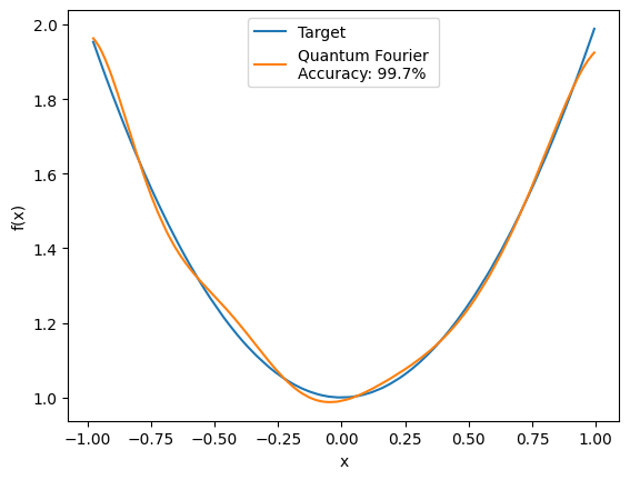
Now we check that Fourier series obtained it’s correct and also fits the function
[8]:
# We import some functions to obtain the Fourier series from the coefficients and to plot these results
from utils_qfiae import fourier_series, plot_data_fourier
# We plot the original function and the Fourier approximation
y_fourier = fourier_series(coeffs, vqr.features)
plot_fourier, accuracy_qnn = plot_data_fourier(vqr.labels * vqr.norm, vqr.features, y_fourier)
4. Integrating every trigonometric piece#
First we should rewrite the Fourier coefficients in a way that will be easy to integrate the trigonometric functions Sine and Cosine
[9]:
# We import some functions to convert exponential-like Fourier coefficients into trigonometric-like and to
# convert this trigonometric coeffs into an array that provides insight about if we get a Sine or a Cosine
from utils_qfiae import exp_fourier_to_trig, trig_to_final_array
trig_coeffs = exp_fourier_to_trig(coeffs)
fourier_array = trig_to_final_array(trig_coeffs)
Let’s visualize what we have and note that in the first columnn 0 stands for Cosine and 1 stands for Sine, in the second column we have the frequencies and in the third one the coefficients
[10]:
print(fourier_array)
[[ 0.00000000e+00  0.00000000e+00  9.91228857e-01]
 [ 0.00000000e+00  1.00000000e+00 -1.82830486e-03]
 [ 0.00000000e+00  2.00000000e+00  6.81657041e-01]
 [ 0.00000000e+00  3.00000000e+00 -3.54067907e-01]
 [ 0.00000000e+00  4.00000000e+00 -7.26099574e-01]
 [ 0.00000000e+00  5.00000000e+00  1.46603674e-01]
 [ 0.00000000e+00  6.00000000e+00  4.57153911e-01]
 [ 0.00000000e+00  7.00000000e+00 -4.26062419e-03]
 [ 0.00000000e+00  8.00000000e+00 -3.14788097e-01]
 [ 0.00000000e+00  9.00000000e+00  1.04707816e-01]
 [ 0.00000000e+00  1.00000000e+01  1.06135314e-02]
 [ 1.00000000e+00  1.00000000e+00  8.67369616e-02]
 [ 1.00000000e+00  2.00000000e+00  4.61132575e-02]
 [ 1.00000000e+00  3.00000000e+00 -2.21834947e-03]
 [ 1.00000000e+00  4.00000000e+00 -2.43216317e-01]
 [ 1.00000000e+00  5.00000000e+00  1.16620823e-01]
 [ 1.00000000e+00  6.00000000e+00  2.77590597e-01]
 [ 1.00000000e+00  7.00000000e+00 -3.20692363e-01]
 [ 1.00000000e+00  8.00000000e+00  6.26751169e-02]
 [ 1.00000000e+00  9.00000000e+00  4.54042108e-02]
 [ 1.00000000e+00  1.00000000e+01  2.90337531e-03]]
Before implementeing the IQAE model, we should define the quantum circuits \(\mathcal{A}\) and \(\mathcal{Q}\).
The circuit \(\mathcal{A}\) is defined as:
where \(a\in[0,1]\) is the parameter to be estimated, while \(|\tilde{\psi}_1\rangle\) and \(|\tilde{\psi}_0\rangle\) are the \(n\)-qubit good and bad states, respectively.
From a more practical point of view, this circuit can be decomposed in two pieces:
where \(\mathcal{I}_1\) is the identity matrix acting over the last qubit.
So, to get \(\mathcal{A}\) we have to define the operator \(\mathcal{P}\), which encodes the probability distribution \(p(x)\), and the operator \(\mathcal{R}\), which encodes the function we are going to integrate, \(\sin(x)^2\), into the interval \([b_{min},b_{max}]\)
[11]:
def operator_p(circ, list_of_qubits):
    """Generating the uniform probability distribution p(x)=1/2^n"""

    for qubit in list_of_qubits:
        circ.add(gates.H(q=qubit))

def operator_r(circ, list_of_qubits, qubit_to_measure, b_max, b_min):
    """Encoding the function Sin(x)^2 to be integrated in the interval [b_min,b_max]"""

    number_of_qubits = qubit_to_measure
    circ.add(
        gates.RY(q=qubit_to_measure, theta=(b_max - b_min) / 2 ** number_of_qubits + 2 * b_min)
    )
    for qubit in list_of_qubits:
        circ.add(
            gates.CRY(qubit, qubit_to_measure,
                      (b_max - b_min) / 2 ** (number_of_qubits-qubit-1))
        )
Then, the circuit \(\mathcal{A}\) will be:
[12]:
def create_circuit_a(n_qubits, b_max, b_min):
    """Creation of circuit A"""

    circuit_a = Circuit(n_qubits + 1)
    list_of_qubits = list(range(n_qubits))
    operator_p(circuit_a, list_of_qubits)
    operator_r(circuit_a, list_of_qubits, n_qubits, b_max, b_min)
    return circuit_a
Let’s see how the circuit A looks like for \(n_{qubits}\)=4
[13]:
circuit_a_prob = create_circuit_a(n_qubits = 4,b_max = x_max_int, b_min = x_min_int)
circuit_a_prob.draw()
q0: ─H──o───────────
q1: ─H──|──o────────
q2: ─H──|──|──o─────
q3: ─H──|──|──|──o──
q4: ─RY─RY─RY─RY─RY─
On the other hand, the circuit \(\mathcal{Q}\) is defined as:
where the operator \(S_0\) tags with a negative sign the \(|0\rangle_{n+1}\) state and does nothing to the other states, and the operator \(S_\chi\) changes the sign to the good state, i.e. \(S_\chi |\tilde{\psi}_1\rangle|1\rangle=-|\tilde{\psi}_1\rangle|1\rangle\).
So, let’s define \(S_0\) and \(S_\chi\) to get \(\mathcal{Q}\):
[14]:
def operator_s_0(circ, qubit_to_measure):
    """Tagging with a negative sign any state different to |0>_{n+1}. Note that this is
    the opposite of what S_0 is supposed to do. The explanation is that the operator
    here defined has absorbed the minus sign in \mathcal{Q}."""

    circ.add(gates.Z(q = qubit_to_measure))

def operator_s_chi(circ, qubit_to_measure):
    """Computing reflection operator (I - 2|0><0|)"""

    number_of_qubits = qubit_to_measure
    list_of_qubits = list(range(number_of_qubits))
    for qubit in list_of_qubits:
        circ.add(gates.X(q = qubit))
    circ.add(gates.X(q=qubit_to_measure))
    circ.add(gates.Z(qubit_to_measure).controlled_by(*range(0,qubit_to_measure)))
    circ.add(gates.X(q=qubit_to_measure))
    for qubit in list_of_qubits:
        circ.add(gates.X(q = qubit))
Then the circuit \(\mathcal{Q}\) will be:
[15]:
def create_circuit_q(n_qubits, circuit_a):
    """Creation of circuit Q"""

    circuit_q = Circuit(n_qubits + 1)
    operator_s_0(circuit_q, n_qubits)
    circuit_q.add(circuit_a.invert().on_qubits(
                    *range(0, n_qubits + 1, 1)))
    operator_s_chi(circuit_q, n_qubits)
    circuit_q.add(circuit_a.on_qubits(
                    *range(0, n_qubits + 1, 1)))
    return circuit_q
Let’s see how the circuit Q looks like for \(n_{qubits}\)=4
[16]:
create_circuit_q(n_qubits=4,circuit_a=circuit_a_prob).draw()
q0: ────────────o──H──X─o─X─H──o───────────
q1: ─────────o──|──H──X─o─X─H──|──o────────
q2: ──────o──|──|──H──X─o─X─H──|──|──o─────
q3: ───o──|──|──|──H──X─o─X─H──|──|──|──o──
q4: ─Z─RY─RY─RY─RY─RY─X─Z─X─RY─RY─RY─RY─RY─
Since we already have the circuits \(\mathcal{A}\) and \(\mathcal{Q}\), we can proceed to execute the IQAE model.
But first let’s do the last transformation of the Fourier coefficients
[17]:
from utils_qfiae import coeffs_array_to_class
coeffs_class = coeffs_array_to_class(fourier_array)
Then, we will create the following function that will integrate each sine and cosine and then sum every term to obtain the final Monte Carlo integral.
To create this integrator we will use the following mathematical properties:
\begin{equation} \frac{1}{x_{min}-x_{min}}\int_{x_{min}}^{x_{max}}dx\sin(x \omega/2)^2=\frac{1}{b_{max}-b_{min}} \int_{b_{min}}^{b_{max}}dx\sin(x)^2, \tag{1} \end{equation}
if \(b_{max}=x_{max}\omega / 2\) and \(b_{min}=x_{min} \omega / 2\).
\begin{equation} \sin(x) = \cos (x - \pi/2) \tag{2} \end{equation}
\begin{equation} \cos(x) = 1 - 2 \sin(x/2) ^ 2 \tag{3} \end{equation}
[18]:
def qfiae_integrator(coeffs_f, x_max, x_min, nbit, shots, alpha, epsilon, method):
    """Takes the Fourier coefficients of the desired function and calculates the integral of the function
    in the specified interval."""

    mc_integral = 0
    error_iqae = 0
    if coeffs_f[0].angle == 0:
        mc_integral += coeffs_f[0].coeff * (x_max - x_min)
    for n in range(1,len(coeffs_f)):
        angle = coeffs_f[n].angle
        if coeffs_f[n].function == 0:  # cosine
            # Here we use Eq.(1)
            a_circuit = create_circuit_a(n_qubits=nbit,
                                         b_max=x_max * angle / 2,
                                         b_min=x_min * angle / 2)

        if coeffs_f[n].function == 1:  # sine
            # Here we use Eq.(2)
            a_circuit = create_circuit_a(n_qubits=nbit,
                                         b_max=x_max * angle / 2 - np.pi / 4,
                                         b_min=x_min * angle / 2 - np.pi / 4)

        q_circuit = create_circuit_q(n_qubits=nbit, circuit_a=a_circuit)
        result = IQAE(a_circuit, q_circuit, alpha, epsilon, n_shots=shots, method=method).execute()
        a_estimated = result.estimation
        # This `a_estimated` corresponds to the integral of the right part of Eq.(1)
        error = result.epsilon_estimated
        # Here we use Eq.(3) and multiply the result by (x_max - x_min) to get rid of the normalization
        mc_integral += (1 - 2 * a_estimated) * coeffs_f[n].coeff * (x_max - x_min)
        error_iqae += (2 * abs(coeffs_f[n].coeff) * error * (x_max - x_min))**2

    return mc_integral , np.sqrt(error_iqae)
Finally, we define the parameters for the IQAE model and execute the qfiae_integrator function
[19]:
nqubits = 4
nshots = 1024
alpha = 0.05
epsilon = 0.005
method_iqae = "chernoff"
qfiae_integral, iae_error = qfiae_integrator(coeffs_class, x_max=x_max_int, x_min=x_min_int,
                                            nbit=nqubits, shots=nshots, alpha=alpha,
                                            epsilon=epsilon, method=method_iqae)
Once the QFIAE algorithm has been performed we can visualize and compare the results with the ones obtained by classical calculation
[20]:
from scipy.integrate import quad
classical_integral, classical_error = quad(f, x_min_int, x_max_int)
print("The result obtained with QFIAE is", qfiae_integral,
      " ± ", iae_error)
print("The result obtained with classical numerical integration is",
      classical_integral, " ± ", classical_error)
The result obtained with QFIAE is 1.3368772283309165  ±  0.00781780414187758
The result obtained with classical numerical integration is 1.3333333333333333  ±  1.4802973661668752e-14