Double-Bracket Iteration diagonalization algorithm#
In this example we present the Qibo’s implementation of the Double-Bracket Iteration (DBI) algorithm, which can be used to prepare the eigenstates of a quantum system.
The initial setup#
At first we import some useful packages.
[1]:
# uncomment this line if seaborn is not installed
# !python -m pip install seaborn
[2]:
from copy import deepcopy

import numpy as np
import matplotlib.pyplot as plt
import seaborn as sns

import optuna

from qibo import hamiltonians, set_backend
from qibo.models.dbi.double_bracket import DoubleBracketGeneratorType, DoubleBracketIteration, DoubleBracketScheduling
Here we define a simple plotting function useful to keep track of the diagonalization process.
[3]:
def visualize_matrix(matrix, title=""):
    """Visualize hamiltonian in a heatmap form."""
    fig, ax = plt.subplots(figsize=(5,5))
    ax.set_title(title)
    try:
        im = ax.imshow(np.absolute(matrix), cmap="inferno")
    except TypeError:
        im = ax.imshow(np.absolute(matrix.get()), cmap="inferno")
    fig.colorbar(im, ax=ax)

def visualize_drift(h0, h):
    """Visualize drift of the evolved hamiltonian w.r.t. h0."""
    fig, ax = plt.subplots(figsize=(5,5))
    ax.set_title(r"Drift: $|\hat{H}_0 - \hat{H}_{\ell}|$")
    try:
        im = ax.imshow(np.absolute(h0 - h), cmap="inferno")
    except TypeError:
        im = ax.imshow(np.absolute((h0 - h).get()), cmap="inferno")

    fig.colorbar(im, ax=ax)

def plot_histories(histories, labels):
    """Plot off-diagonal norm histories over a sequential evolution."""
    colors = sns.color_palette("inferno", n_colors=len(histories)).as_hex()
    plt.figure(figsize=(5,5*6/8))
    for i, (h, l) in enumerate(zip(histories, labels)):
        plt.plot(h, lw=2, color=colors[i], label=l, marker='.')
    plt.legend()
    plt.xlabel("Iterations")
    plt.ylabel(r"$\| \sigma(\hat{H}) \|^2$")
    plt.title("Loss function histories")
    plt.grid(True)
    plt.show()
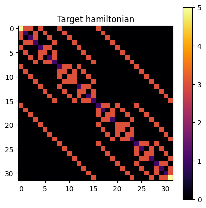
We need to define a target hamiltonian which we aim to diagonalize. As an example, we consider the Transverse Field Ising Model (TFIM):
which is already implemented in Qibo. For this tutorial we set \(N=6\) and \(h=3\).
[4]:
# set the qibo backend (we suggest qibojit if N >= 20)
set_backend("numpy")

# hamiltonian parameters
nqubits = 5
h = 3

# define the hamiltonian
h = hamiltonians.TFIM(nqubits=nqubits, h=h)

# vosualize the matrix
visualize_matrix(h.matrix, title="Target hamiltonian")
[Qibo 0.2.12|INFO|2024-09-06 12:03:17]: Using numpy backend on /CPU:0
The generator of the evolution#
The model is implemented following the procedure presented in [1], and the first practical step is to define the generator of the iteration \(\hat{\mathcal{U}}_{\ell}\), which executes one diagonalization step
In Qibo, we define the iteration type through a DoubleBracketGeneratorType object, which can be chosen between one of the following: - canonical: the generator of the iteration at step \(k+1\) is defined using the commutator between the off diagonal part \(\sigma(\hat{H_k})\) and the diagonal part \(\Delta(\hat{H}_k)\) of the target evolved hamiltonian:
single_commutator: the evolution follows a similar procedure of the previous point in this list, but any additional matrix \(D_k\) can be used to control the evolution at each step:
group_commutator: the following group commutator is used to compute the evolution:
which approximates the canonical commutator for small \(s\).
In order to set one of this evolution generators one can do as follow:
[5]:
# we have a look inside the DoubleBracketGeneratorType class
for generator in DoubleBracketGeneratorType:
    print(generator)
DoubleBracketGeneratorType.canonical
DoubleBracketGeneratorType.single_commutator
DoubleBracketGeneratorType.group_commutator
DoubleBracketGeneratorType.group_commutator_third_order
[6]:
# here we set the canonical generator
iterationtype = DoubleBracketGeneratorType.canonical
The DoubleBracketIteration class#
A DoubleBracketIteration object can be initialize by calling the qibo.models.double_braket.DoubleBracketIteration model and passing the target hamiltonian and the generator type we want to use to perform the evolutionary steps.
[7]:
dbf = DoubleBracketIteration(hamiltonian=deepcopy(h), mode=iterationtype)
DoubleBracketIteration features#
[8]:
# on which qibo backend am I running the algorithm?
print(f"Backend: {dbf.backend}")
Backend: numpy
[9]:
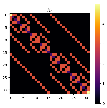
# the initial target hamiltonian is a qibo hamiltonian
# thus the matrix can be accessed typing h.matrix
print(f"Initial form of the target hamiltonian:\n{dbf.h0.matrix}")
Initial form of the target hamiltonian:
[[-5.-0.j -3.-0.j -3.-0.j ... -0.-0.j -0.-0.j -0.-0.j]
 [-3.-0.j -1.-0.j -0.-0.j ... -0.-0.j -0.-0.j -0.-0.j]
 [-3.-0.j -0.-0.j -1.-0.j ... -0.-0.j -0.-0.j -0.-0.j]
 ...
 [-0.-0.j -0.-0.j -0.-0.j ... -1.-0.j -0.-0.j -3.-0.j]
 [-0.-0.j -0.-0.j -0.-0.j ... -0.-0.j -1.-0.j -3.-0.j]
 [-0.-0.j -0.-0.j -0.-0.j ... -3.-0.j -3.-0.j -5.-0.j]]
[10]:
# let's visualize it in a more graphical way
visualize_matrix(dbf.h0.matrix, r"$H_0$")
[11]:
# since we didn't perform yet any evolutionary step they are the same
visualize_drift(dbf.h0.matrix, dbf.h.matrix)
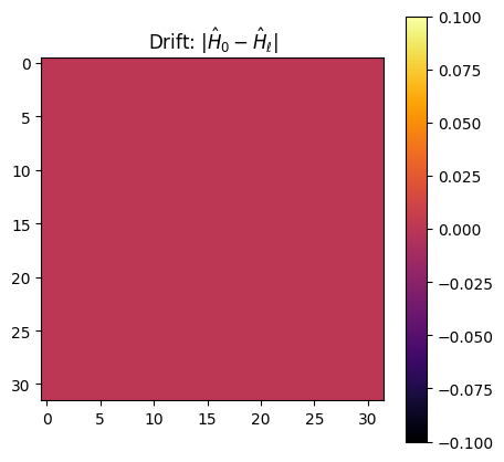
which shows \(\hat{H}\) is now identical to \(\hat{H}_0\) since no evolution step has been performed yet.
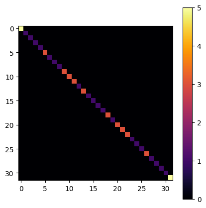
[12]:
# diagonal part of the H target
visualize_matrix(dbf.diagonal_h_matrix)
The Hilbert-Schmidt norm of a Hamiltonian is defined as:
\(\langle A\rangle_{HS}=\sqrt{A^\dagger A}\)
[13]:
# Hilbert-Schmidt norm of the off-diagonal part
# which we want to bring to be close to zero
print(f"HS norm of the off diagonal part of H: {dbf.off_diagonal_norm}")
HS norm of the off diagonal part of H: 37.94733192202055
Finally, the energy fluctuation of the system at step \(k\) over a given state \(\mu\)
can be computed:
[14]:
# define a quantum state
# for example the ground state of a multi-qubit Z hamiltonian
Z = hamiltonians.Z(nqubits=nqubits)
state = Z.ground_state()

# compute energy fluctuations using current H and given state
dbf.energy_fluctuation(state)
[14]:
6.708203932499369
Call the DoubleBracketIteration to perform a DBF iteration#
If the DBF object is called, a Double Bracket Iteration iteration is performed. This can be done customizing the iteration by setting the iteration step and the desired DoubleBracketGeneratorType. If no generator is provided, the one passed at the initialization time is used (default is DoubleBracketGeneratorType.canonical).
[15]:
# perform one evolution step

# initial value of the off-diagonal norm
print(f"Initial value of the off-diagonal norm: {dbf.off_diagonal_norm}")

dbf(step=0.01, mode=iterationtype)

# after one step
print(f"One step later off-diagonal norm: {dbf.off_diagonal_norm}")
Initial value of the off-diagonal norm: 37.94733192202055
One step later off-diagonal norm: 34.179717587686405
We can check now if something happened by plotting the drift:
[16]:
visualize_drift(dbf.h0.matrix, dbf.h.matrix)
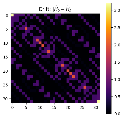
The set step can be good, but maybe not the best one. In order to do this choice in a wiser way, we can call the DBF hyperoptimization routine to search for a better initial step. The dbf.hyperopt_step method is built on top of the `hyperopt <https://hyperopt.github.io/hyperopt/>`__ package. Any algorithm or sampling space provided by the official package can be used. We are going to use the default options (we sample new steps from a uniform space following a Tree of Parzen estimators
algorithm).
[17]:
# restart
dbf.h = dbf.h0

# optimization of the step, we allow to search in [1e-5, 1]
step = dbf.choose_step(
    scheduling=DoubleBracketScheduling.hyperopt,
    step_min = 1e-5,
    step_max = 1,
    optimizer = optuna.samplers.TPESampler(),
    max_evals = 1000,
)
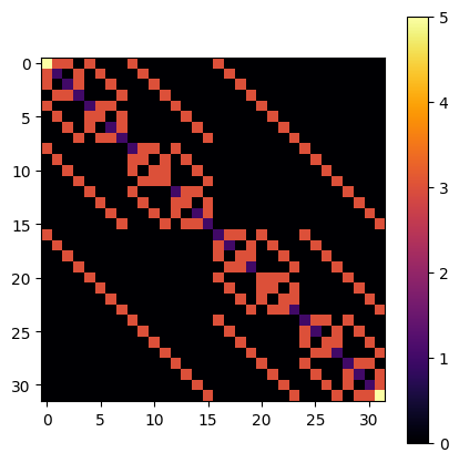
[18]:
visualize_matrix(dbf.h.matrix)
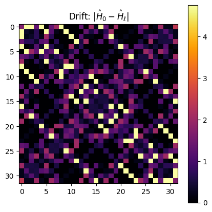
[19]:
visualize_drift(dbf.h0.matrix, dbf.h.matrix)
Let’s evolve the model for NSTEPS#
We know recover the initial hamiltonian, and we perform a sequence of DBF iteration steps, in order to show how this mechanism can lead to a proper diagonalization of the target hamiltonian.
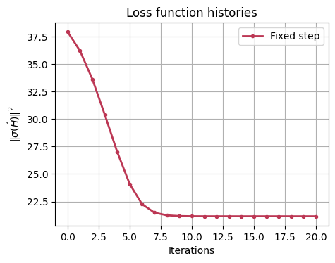
Method 1: fixed step#
[20]:
# restart
dbf_1 = DoubleBracketIteration(hamiltonian=deepcopy(h), mode=iterationtype)
off_diagonal_norm_history = [dbf_1.off_diagonal_norm]
histories, labels = [], ["Fixed step"]

# set the number of evolution steps
NSTEPS = 20
step = 0.005

for s in range(NSTEPS):
    dbf_1(step=step)
    off_diagonal_norm_history.append(dbf_1.off_diagonal_norm)

histories.append(off_diagonal_norm_history)
[21]:
plot_histories(histories, labels)
Method 2: optimizing the step#
[23]:
# restart
dbf_2 = DoubleBracketIteration(hamiltonian=deepcopy(h), mode=iterationtype, scheduling=DoubleBracketScheduling.hyperopt)
off_diagonal_norm_history = [dbf_2.off_diagonal_norm]

# set the number of evolution steps
NSTEPS = 20

# optimize first step
step = dbf_2.choose_step(
    step_min = 1e-5,
    step_max = 1,
    optimizer = optuna.samplers.TPESampler(),
    max_evals = 1000,
)

for s in range(NSTEPS):
    if s != 0:
        step = dbf_2.choose_step(
            step_min = 1e-5,
            step_max = 1,
            optimizer = optuna.samplers.TPESampler(),
            max_evals = 1000,
        )
        print(f"New optimized step at iteration {s}/{NSTEPS}: {step}")
    dbf_2(step=step)
    off_diagonal_norm_history.append(dbf_2.off_diagonal_norm)

histories.append(off_diagonal_norm_history)
labels.append("Optimizing step")
New optimized step at iteration 1/20: 0.00934294935664311
New optimized step at iteration 2/20: 0.009364588177233102
New optimized step at iteration 3/20: 0.005985356940597437
New optimized step at iteration 4/20: 0.011472840984366184
New optimized step at iteration 5/20: 0.006802887431910996
New optimized step at iteration 6/20: 0.010837702507351613
New optimized step at iteration 7/20: 0.006624471861894687
New optimized step at iteration 8/20: 0.00870720701470905
New optimized step at iteration 9/20: 0.005748706054245771
New optimized step at iteration 10/20: 0.009512049459920756
New optimized step at iteration 11/20: 0.004887478565382978
New optimized step at iteration 12/20: 0.011309993175156744
New optimized step at iteration 13/20: 0.0017896288977535153
New optimized step at iteration 14/20: 0.0003944795659594491
New optimized step at iteration 15/20: 0.0006390700306615794
New optimized step at iteration 16/20: 0.0008772593599309826
New optimized step at iteration 17/20: 0.012559015937191706
New optimized step at iteration 18/20: 0.003294180889937215
New optimized step at iteration 19/20: 0.002707744316510693
[24]:
plot_histories(histories, labels)
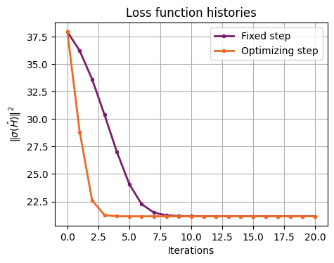
The hyperoptimization can lead to a faster convergence of the algorithm.
[25]:
visualize_matrix(dbf_1.h.matrix)
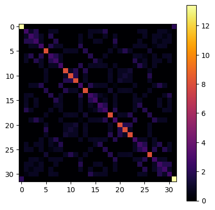
[26]:
visualize_matrix(dbf_2.h.matrix)

[ ]: