Models#
Qibo provides models for both the circuit based and the adiabatic quantum
computation paradigms. Circuit based models include Circuit models which
allow defining arbitrary circuits and Quantum Fourier Transform (QFT) such as the
Quantum Fourier Transform (qibo.models.QFT) and the
Variational Quantum Eigensolver (qibo.models.VQE).
Adiabatic quantum computation is simulated using the Time evolution
of state vectors.
In order to perform calculations and apply gates to a state vector a backend
has to be used. The backends are defined in qibo/backends.
Circuit and gate objects are backend independent and can be executed with
any of the available backends.
Qibo uses big-endian byte order, which means that the most significant qubit is the one with index 0, while the least significant qubit is the one with the highest index.
Circuit models#
Circuit#
- class qibo.models.circuit.Circuit(nqubits: int | list | None = None, accelerators: dict | None = None, density_matrix: bool = False, wire_names: list | None = None)[source]#
Circuit object which holds a list of gates.
This circuit is symbolic and cannot perform calculations. A specific backend has to be used for performing calculations.
Circuits can be created with a specific number of qubits and wire names.
Either
nqubitsorwire_namesmust be provided.If only
nqubitsis provided, wire names will default to[0, 1, ..., nqubits - 1].If only
wire_namesis provided,nqubitswill be set to the length ofwire_names.nqubitsandwire_namesmust be consistent with each other.
Example:
from qibo import Circuit

# Every circuit initialization below is valid
circuit = Circuit(5)  # Default wire names are [0, 1, 2, 3, 4]
circuit = Circuit(["A", "B", "C", "D", "E"])
circuit = Circuit(5, wire_names=["A", "B", "C", "D", "E"])
circuit = Circuit(wire_names=["A", "B", "C", "D", "E"])
- Parameters:
nqubits (int | list, optional) – Number of qubits in the circuit or a list of wire names.
wire_names (list, optional) – List of wire names
init_kwargs (dict) –
a dictionary with the following keys
nqubits
accelerators
density_matrix
wire_names.
queue (_Queue) – List that holds the queue of gates of a circuit.
parametrized_gates (_ParametrizedGates) – List of parametric gates.
trainable_gates (_ParametrizedGates) – List of trainable gates.
measurements (list) – List of non-collapsible measurements.
_final_state – Final result after full simulation of the circuit.
compiled (CompiledExecutor) – Circuit executor. Defaults to
None.repeated_execution (bool) – If True, the circuit would be re-executed when sampling. Defaults to
False.density_matrix (bool, optional) – If True, the circuit would evolve density matrices. If
False, defaults to statevector simulation. Defaults toFalse.accelerators (dict, optional) – Dictionary that maps device names to the number of times each device will be used. Defaults to
None.ndevices (int) – Total number of devices. Defaults to
None.nglobal (int) – Base two logarithm of the number of devices. Defaults to
None.nlocal (int) – Total number of available qubits in each device. Defaults to
None.queues (DistributedQueues) – Gate queues for each accelerator device. Defaults to
None.
- on_qubits(*qubits)[source]#
Generator of gates contained in the circuit acting on specified qubits.
Useful for adding a circuit as a subroutine in a larger circuit.
- Parameters:
qubits (int) – Qubit ids that the gates should act.
Example
from qibo import Circuit, gates

# create small circuit on 4 qubits
small_circuit = Circuit(4)
small_circuit.add(gates.RX(qubit, theta=0.1) for qubit in range(4))
small_circuit.add((gates.CNOT(0, 1), gates.CNOT(2, 3)))
# create large circuit on 8 qubits
large_circuit = Circuit(8)
large_circuit.add(gates.RY(qubit, theta=0.1) for qubit in range(8))
# add the small circuit to the even qubits of the large one
large_circuit.add(small_circuit.on_qubits(*range(0, 8, 2)))
- light_cone(*qubits)[source]#
Reduces circuit to the qubits relevant for an observable.
Useful for calculating expectation values of local observables without requiring simulation of large circuits. Uses the light cone construction described in issue #571.
- Parameters:
qubits (int) – Qubit ids that the observable has support on.
- Returns:
- Circuit that contains only
the qubits that are required for calculating expectation involving the given observable qubits.
- qubit_map (dict): Dictionary mapping the qubit ids of the original
circuit to the ids in the new one.
- Return type:
circuit (
qibo.models.Circuit)
- copy(deep: bool = False)[source]#
Creates a copy of the current
circuitas a newCircuitmodel.- Parameters:
deep (bool) – If
Truecopies of the gate objects will be created for the new circuit. IfFalse, the same gate objects ofcircuitwill be used.- Returns:
The copied circuit object.
- invert()[source]#
Creates a new
Circuitthat is the inverse of the original.Inversion is obtained by taking the dagger of all gates in reverse order. If the original circuit contains parametrized gates, dagger will change their parameters. This action is not persistent, so if the parameters are updated afterwards, for example using
qibo.models.circuit.Circuit.set_parameters(), the action of dagger will be overwritten. If the original circuit contains measurement gates, these are included in the inverted circuit.- Returns:
Circuit corresponding to the inverse of the original
circuit.- Return type:
qibo.models.Circuit
- decompose(*free: int, method: str = 'standard', **kwargs)[source]#
Decomposes circuit’s gates to gates supported by OpenQASM.
- Parameters:
free (int) – Ids of free (work) qubits to use for gate decomposition.
method (str, optional) – Choice of gate set for the decomposition. If
"standard", decomposes circuit intoqibo.gates.gates.CNOT,qibo.gates.gates.RX,qibo.gates.gates.RY,qibo.gates.gates.RZ,qibo.gates.gates.U1,qibo.gates.gates.U2,qibo.gates.gates.U3, and Clifford gates. If"clifford_plus_t", decomposes the circuit intoqibo.gates.gates.CNOT,qibo.gates.gates.H,qibo.gates.gates.S,qibo.gates.gates.X,qibo.gates.gates.Y,qibo.gates.gates.Z, andqibo.gates.gates.T. Defaults to"standard".
- Returns:
Circuit that contains only gates that are supported by OpenQASM and has the same effect as the original circuit.
- Return type:
- with_pauli_noise(noise_map: Tuple[int, int, int] | Dict[int, Tuple[int, int, int]])[source]#
Creates a copy of the circuit with Pauli noise gates after each gate.
If the original circuit uses state vectors then noise simulation will be done using sampling and repeated circuit execution. In order to use density matrices the original circuit should be created setting the flag
density_matrix=True. For more information we refer to the How to perform noisy simulation? example.- Parameters:
noise_map (dict) – list of tuples \((P_{k}, p_{k})\), where \(P_{k}\) is a
strrepresenting the \(k\)-th \(n\)-qubit Pauli operator, and \(p_{k}\) is the associated probability.- Returns:
Circuit object that contains all the gates of the original circuit and additional noise channels on all qubits after every gate.
Example
from qibo import Circuit, gates
# use density matrices for noise simulation
circuit = Circuit(2, density_matrix=True)
circuit.add([gates.H(0), gates.H(1), gates.CNOT(0, 1)])
noise_map = {
    0: list(zip(["X", "Z"], [0.1, 0.2])),
    1: list(zip(["Y", "Z"], [0.2, 0.1]))
}
noisy_circuit = circuit.with_pauli_noise(noise_map)
# ``noisy_circuit`` will be equivalent to the following circuit
circuit_2 = Circuit(2, density_matrix=True)
circuit_2.add(gates.H(0))
circuit_2.add(gates.PauliNoiseChannel(0, [("X", 0.1), ("Z", 0.2)]))
circuit_2.add(gates.H(1))
circuit_2.add(gates.PauliNoiseChannel(1, [("Y", 0.2), ("Z", 0.1)]))
circuit_2.add(gates.CNOT(0, 1))
circuit_2.add(gates.PauliNoiseChannel(0, [("X", 0.1), ("Z", 0.2)]))
circuit_2.add(gates.PauliNoiseChannel(1, [("Y", 0.2), ("Z", 0.1)]))
- add(gate: Gate)[source]#
Add a gate to a given queue.
- Parameters:
gate (
qibo.gates.Gate) – the gate object to add. See Gates for a list of available gates. gate can also be an iterable or generator of gates. In this case all gates in the iterable will be added in the circuit.- Returns:
If the circuit contains measurement gates with
collapse=Trueasympy.Symbolthat parametrizes the corresponding outcome.
- gates_of_type(gate: str | type) List[Tuple[int, Gate]][source]#
Finds all gate objects of specific type or name.
This method can be affected by how
qibo.gates.Gate.controlled_by()behaves with certain gates. To see howqibo.gates.Gate.controlled_by()affects gates, we refer to the documentation ofqibo.gates.Gate.controlled_by().
- set_parameters(parameters: List[float] | Dict[str, float] | _Buffer | _SupportsArray[dtype[Any]] | _NestedSequence[_SupportsArray[dtype[Any]]] | bool | int | float | complex | str | bytes | _NestedSequence[bool | int | float | complex | str | bytes]) None[source]#
Updates the parameters of the circuit’s parametrized gates.
For more information on how to use this method we refer to the How to use parametrized gates? example.
- Parameters:
parameters – Container holding the new parameter values. It can have one of the following types: List with length equal to the number of parametrized gates and each of its elements compatible with the corresponding gate. Dictionary with keys that are references to the parametrized gates and values that correspond to the new parameters for each gate. Flat list with length equal to the total number of free parameters in the circuit. A backend supported tensor (for example
np.ndarrayortf.Tensor) may also be given instead of a flat list.
Example
from qibo import Circuit, gates
# create a circuit with all parameters set to 0.
circuit = Circuit(3)
circuit.add(gates.RX(0, theta=0))
circuit.add(gates.RY(1, theta=0))
circuit.add(gates.CZ(1, 2))
circuit.add(gates.fSim(0, 2, theta=0, phi=0))
circuit.add(gates.H(2))

# set new values to the circuit's parameters using list
params = [0.123, 0.456, (0.789, 0.321)]
circuit.set_parameters(params)
# or using dictionary
params = {
    circuit.queue[0]: 0.123,
    circuit.queue[1]: 0.456,
    circuit.queue[3]: (0.789, 0.321)
}
circuit.set_parameters(params)
# or using flat list (or an equivalent `np.array`/`tf.Tensor`/`torch.Tensor`)
params = [0.123, 0.456, 0.789, 0.321]
circuit.set_parameters(params)
- get_parameters(output_format: str = 'list', include_not_trainable: bool = False) List | Dict[source]#
Returns the parameters of all parametrized gates in the circuit.
Inverse method of
qibo.models.circuit.Circuit.set_parameters().- Parameters:
output_format (str) – Format to return the variational parameters. Available formats are
"list","dict"and"flatlist". Seeqibo.models.circuit.Circuit.set_parameters()for more details on each format. Default is"list".include_not_trainable (bool) – If
Trueit includes the parameters of non-trainable parametrized gates in the returned list or dictionary. Default isFalse.
- associate_gates_with_parameters() List[Gate][source]#
Associates to each parameter its gate.
- Returns:
A nparams-long flatlist whose i-th element is the gate parameterized by the i-th parameter.
- summary() None[source]#
Display a summary of the circuit.
The summary contains the circuit depths, total number of qubits and the all gates sorted in decreasing number of appearance.
Example
- fuse(max_qubits: int = 2)[source]#
Creates an equivalent circuit by fusing gates for increased simulation performance.
- Parameters:
max_qubits (int) – Maximum number of qubits in the fused gates.
- Returns:
A
qibo.core.circuit.Circuitobject containingqibo.gates.FusedGategates, each of which corresponds to a group of some original gates. For more details on the fusion algorithm we refer to the Circuit fusion section.
Example
from qibo import Circuit, gates

circuit = Circuit(2)
circuit.add([gates.H(0), gates.H(1)])
circuit.add(gates.CNOT(0, 1))
circuit.add([gates.Y(0), gates.Y(1)])
# create circuit with fused gates
fused_circuit = circuit.fuse()
# now ``fused_circuit`` contains a single ``FusedGate`` that is
# equivalent to applying the five original gates
- unitary(backend: Backend | None = None) _Buffer | _SupportsArray[dtype[Any]] | _NestedSequence[_SupportsArray[dtype[Any]]] | bool | int | float | complex | str | bytes | _NestedSequence[bool | int | float | complex | str | bytes][source]#
Creates the unitary matrix corresponding to all circuit gates.
This is a \(2^{n} \times 2^{n}`\) matrix obtained by multiplying all circuit gates, where \(n\) is
nqubits.
- property final_state: _Buffer | _SupportsArray[dtype[Any]] | _NestedSequence[_SupportsArray[dtype[Any]]] | bool | int | float | complex | str | bytes | _NestedSequence[bool | int | float | complex | str | bytes]#
Returns the final state after full simulation of the circuit.
If the circuit is executed more than once, only the last final state is returned.
- execute(initial_state: _Buffer | _SupportsArray[dtype[Any]] | _NestedSequence[_SupportsArray[dtype[Any]]] | bool | int | float | complex | str | bytes | _NestedSequence[bool | int | float | complex | str | bytes] = None, nshots: int = 1000, **kwargs)[source]#
Executes the circuit. Exact implementation depends on the backend.
- Parameters:
initial_state (ndarray or
qibo.models.circuit.Circuit) – Initial configuration. It can be specified by the setting the state vector using an array or a circuit. IfNone, the initial state is|000..00>.nshots (int, optional) – Number of shots. Defaults ot \(1000\).
- Returns:
Either a
qibo.result.QuantumState,qibo.result.MeasurementOutcomesorqibo.result.CircuitResultdepending on the circuit’s configuration.
- classmethod from_dict(raw: dict)[source]#
Load from serialization.
Essentially the counter-part of
raw().
- to_qasm(extended_compatibility: bool = False) str[source]#
Convert circuit to a QASM string.
- Parameters:
extended_compatibility (bool) – if
True, unrolls more exotic gates in their decomposition by defining them as custom gates, this increases the compatibility with other frameworks, such asqiskit. Defaults toFalse.- Returns:
The generated QASM.
- Return type:
Note
This method does not support multi-controlled gates and gates with
torch.Tensoras parameters.
- classmethod from_qasm(qasm_code: str, **circuit_kwargs)[source]#
Constructs a circuit from QASM code.
- Parameters:
- Returns:
Circuit containing the gates specified by the given QASM script.
- Return type:
Example
from qibo import Circuit, gates
qasm_code = '''OPENQASM 2.0;
include "qelib1.inc";
qreg q[2];
h q[0];
h q[1];
cx q[0],q[1];'''
circuit = Circuit.from_qasm(qasm_code)
# is equivalent to creating the following circuit
circuit_2 = Circuit(2)
circuit_2.add(gates.H(0))
circuit_2.add(gates.H(1))
circuit_2.add(gates.CNOT(0, 1))
- classmethod from_qasm_file(qasm_file: str, **circuit_kwargs)[source]#
Constructs a circuit from QASM code in a
qasm_file.- Parameters:
- Returns:
Circuit containing the gates specified by the given QASM script.
- Return type:
- to_qir()[source]#
Convert circuit to QIR circuit.
Uses qbraid (https://github.com/qBraid/qBraid) to transpile the circuit into pyqir circuits.
- to_cudaq()[source]#
Convert circuit to CUDA-Q (quake) code.
Uses qbraid (https://github.com/qBraid/qBraid) to transpile the circuit into cudaq circuits.
- classmethod from_cudaq(cudaq_circuit_code)[source]#
Construct a circuit from CUDA-Q (quake) code.
Uses qbraid (https://github.com/qBraid/qBraid) to transpile the cudaq circuit into a qibo.models.circuit.Circuit.
- Parameters:
cudaq_circuit_code (PyKernel) – kernel containing the cudaq circuit code.
- Returns:
qibo.models.circuit.Circuitrepresenting the given circuit.
- diagram(line_wrap: int = 70, legend: bool = False) str[source]#
Build the string representation of the circuit diagram.
Circuit addition#
qibo.models.circuit.Circuit objects support addition. For example
circuit_1 = QFT(4)

circuit_2 = Circuit(4)
circuit_2.add(gates.RZ(0, 0.1234))
circuit_2.add(gates.RZ(1, 0.1234))
circuit_2.add(gates.RZ(2, 0.1234))
circuit_2.add(gates.RZ(3, 0.1234))

circuit = circuit_1 + circuit_2
will create a circuit that performs the Quantum Fourier Transform on four qubits followed by Rotation-Z gates.
Circuit fusion#
The gates contained in a circuit can be fused up to two-qubits using the
qibo.models.circuit.Circuit.fuse() method. This returns a new circuit
for which the total number of gates is less than the gates in the original
circuit as groups of gates have been fused to a single
qibo.gates.special.FusedGate gate. Simulating the new circuit
is equivalent to simulating the original one but in most cases more efficient
since less gates need to be applied to the state vector.
The fusion algorithm works as follows: First all gates in the circuit are
transformed to unmarked qibo.gates.special.FusedGate. The gates
are then processed in the order they were added in the circuit. For each gate
we identify the neighbors forth and back in time and attempt to fuse them to
the gate. Two gates can be fused if their total number of target qubits is
smaller than the fusion maximum qubits (specified by the user) and there are
no other gates between acting on the same target qubits. Gates that are fused
to others are marked. The new circuit queue contains the gates that remain
unmarked after the above operations finish.
Gates are processed in the original order given by user. There are no
additional simplifications performed such as commuting gates acting on the same
qubit or canceling gates even when such simplifications are mathematically possible.
The user can specify the maximum number of qubits in a fused gate using
the max_qubits flag in qibo.models.circuit.Circuit.fuse().
For example the following:
from qibo import Circuit, gates

circuit = Circuit(2)
circuit.add([gates.H(0), gates.H(1)])
circuit.add(gates.CZ(0, 1))
circuit.add([gates.X(0), gates.Y(1)])
fused_circuit = circuit.fuse()
will create a new circuit with a single qibo.gates.special.FusedGate
acting on (0, 1), while the following:
from qibo import Circuit, gates

circuit = Circuit(3)
circuit.add([gates.H(0), gates.H(1), gates.H(2)])
circuit.add(gates.CZ(0, 1))
circuit.add([gates.X(0), gates.Y(1), gates.Z(2)])
circuit.add(gates.CNOT(1, 2))
circuit.add([gates.H(0), gates.H(1), gates.H(2)])
fused_circuit = circuit.fuse()
will give a circuit with two fused gates, the first of which will act on
(0, 1) corresponding to
[H(0), H(1), CZ(0, 1), X(0), H(0)]
and the second will act to (1, 2) corresponding to
[Y(1), Z(2), CNOT(1, 2), H(1), H(2)]
Quantum Fourier Transform (QFT)#
- class qibo.models.qft.QFT(nqubits: int, with_swaps: bool = True, accelerators=None, **kwargs)[source]#
Creates a circuit that implements the Quantum Fourier Transform.
- Parameters:
nqubits (int) – number of qubits in the circuit.
with_swaps (bool, optional) – If
True, usesqibo.gates.SWAPgates at the end of the circuit so that the qubit order in the final state is the same as the initial state. Defauts toTrue.accelerators (dict, optional) – Accelerator device dictionary in order to use a distributed circuit. If
None, a simple (non-distributed) circuit will be used.kwargs (dict, optional) – Additional arguments used to initialize
qibo.models.Circuit. For details, see the documentation ofqibo.models.circuit.Circuit.
- Returns:
implementation of the Quantum Fourier Transform.
- Return type:
qibo.models.Circuit
Example
import numpy as np
from qibo.models import QFT
nqubits = 6
circuit = QFT(nqubits)
# Random normalized initial state vector
init_state = np.random.random(2 ** nqubits) + 1j * np.random.random(2 ** nqubits)
init_state = init_state / np.sqrt((np.abs(init_state)**2).sum())
# Execute the circuit
final_state = circuit(init_state)
Variational Quantum Eigensolver (VQE)#
- class qibo.models.variational.VQE(circuit, hamiltonian)[source]#
This class implements the variational quantum eigensolver algorithm.
- Parameters:
circuit (
qibo.models.circuit.Circuit) – Circuit that implements the variaional ansatz.hamiltonian (
qibo.hamiltonians.Hamiltonian) – Hamiltonian object.
Example
import numpy as np

from qibo import Circuit, gates
from qibo.hamiltonians import XXZ
from qibo.models import VQE

# create circuit ansatz for two qubits
circuit = Circuit(2)
circuit.add(gates.RY(0, theta=0))
# create XXZ Hamiltonian for two qubits
hamiltonian = XXZ(2)
# create VQE model for the circuit and Hamiltonian
vqe = VQE(circuit, hamiltonian)
# optimize using random initial variational parameters
initial_parameters = np.random.uniform(0, 2, 1)
vqe.minimize(initial_parameters)
- minimize(initial_state, method='Powell', loss_func=None, jac=None, hess=None, hessp=None, bounds=None, constraints=(), tol=None, callback=None, options=None, compile=False, processes=None)[source]#
Search for parameters which minimizes the hamiltonian expectation.
- Parameters:
initial_state (array) – a initial guess for the parameters of the variational circuit.
method (str) – the desired minimization method. See
qibo.optimizers.optimize()for available optimization methods.loss (callable) – loss function, the default one is
qibo.models.utils.vqe_loss().jac (dict) – Method for computing the gradient vector for scipy optimizers.
hess (dict) – Method for computing the hessian matrix for scipy optimizers.
hessp (callable) – Hessian of objective function times an arbitrary vector for scipy optimizers.
bounds (sequence or Bounds) – Bounds on variables for scipy optimizers.
constraints (dict) – Constraints definition for scipy optimizers.
tol (float) – Tolerance of termination for scipy optimizers.
callback (callable) – Called after each iteration for scipy optimizers.
options (dict) – a dictionary with options for the different optimizers.
compile (bool) – whether the TensorFlow graph should be compiled.
processes (int) – number of processes when using the paralle BFGS method.
- Returns:
The final expectation value. The corresponding best parameters. The optimization result object. For scipy methods it returns the
OptimizeResult, for'cma'theCMAEvolutionStrategy.result, and for'sgd'the options used during the optimization.
Adiabatically Assisted Variational Quantum Eigensolver (AAVQE)#
- class qibo.models.variational.AAVQE(circuit, easy_hamiltonian, problem_hamiltonian, s, nsteps=10, t_max=1, bounds_tolerance=1e-07, time_tolerance=1e-07)[source]#
This class implements the Adiabatically Assisted Variational Quantum Eigensolver algorithm. See https://arxiv.org/abs/1806.02287.
- Parameters:
circuit (
qibo.models.circuit.Circuit) – variational ansatz.easy_hamiltonian (
qibo.hamiltonians.Hamiltonian) – initial Hamiltonian object.problem_hamiltonian (
qibo.hamiltonians.Hamiltonian) – problem Hamiltonian object.s (callable) – scheduling function of time that defines the adiabatic evolution. It must verify boundary conditions: s(0) = 0 and s(1) = 1.
nsteps (float) – number of steps of the adiabatic evolution.
t_max (float) – total time evolution.
bounds_tolerance (float) – tolerance for checking s(0) = 0 and s(1) = 1.
time_tolerance (float) – tolerance for checking if time is greater than t_max.
Example
import numpy as np

from qibo import Circuit, gates
from qibo.hamiltonians import X, XXZ
from qibo.models import AAVQE

# create circuit ansatz for two qubits
circuit = Circuit(2)
circuit.add(gates.RY(0, theta=0))
circuit.add(gates.RY(1, theta=0))
# define the easy and the problem Hamiltonians.
easy_hamiltonian = X(2)
problem_hamiltonian = XXZ(2)
# define a scheduling function with only one parameter
# and boundary conditions s(0) = 0, s(1) = 1
s = lambda t: t
# create AAVQE model
aavqe = AAVQE(
    circuit,
    easy_hamiltonian,
    problem_hamiltonian,
    s,
    nsteps=10,
    t_max=1
)
# optimize using random initial variational parameters
np.random.seed(0)
initial_parameters = np.random.uniform(0, 2*np.pi, 2)
ground_energy, params = aavqe.minimize(initial_parameters)
- minimize(params, method='BFGS', jac=None, hess=None, hessp=None, bounds=None, constraints=(), tol=None, options=None, compile=False, processes=None)[source]#
Performs minimization to find the ground state of the problem Hamiltonian.
- Parameters:
params (np.ndarray or list) – initial guess for the parameters of the variational circuit.
method (str) – optimizer to employ.
jac (dict) – Method for computing the gradient vector for scipy optimizers.
hess (dict) – Method for computing the hessian matrix for scipy optimizers.
hessp (callable) – Hessian of objective function times an arbitrary vector for scipy optimizers.
bounds (sequence or Bounds) – Bounds on variables for scipy optimizers.
constraints (dict) – Constraints definition for scipy optimizers.
tol (float) – Tolerance of termination for scipy optimizers.
options (dict) – a dictionary with options for the different optimizers.
compile (bool) – whether the TensorFlow graph should be compiled.
processes (int) – number of processes when using the parallel BFGS method.
Quantum Approximate Optimization Algorithm (QAOA)#
- class qibo.models.variational.QAOA(hamiltonian, mixer=None, solver='exp', callbacks=[], accelerators=None)[source]#
Quantum Approximate Optimization Algorithm (QAOA) model.
The QAOA is introduced in arXiv:1411.4028.
- Parameters:
hamiltonian (
qibo.hamiltonians.Hamiltonian) – problem Hamiltonian whose ground state is sought.mixer (
qibo.hamiltonians.Hamiltonian) – mixer Hamiltonian. Must be of the same type and act on the same number of qubits ashamiltonian. IfNone,qibo.hamiltonians.Xis used.solver (str) – solver used to apply the exponential operators. Default solver is ‘exp’ (
qibo.solvers.Exponential).callbacks (list) – List of callbacks to calculate during evolution.
accelerators (dict) – Dictionary of devices to use for distributed execution. This option is available only when
hamiltonianis aqibo.hamiltonians.SymbolicHamiltonian.
Example
import numpy as np

from qibo.hamiltonians import XXZ
from qibo.models import QAOA

# create XXZ Hamiltonian for four qubits
hamiltonian = XXZ(4)
# create QAOA model for this Hamiltonian
qaoa = QAOA(hamiltonian)
# optimize using random initial variational parameters
# and default options and initial state
initial_parameters = 0.01 * np.random.random(4)
best_energy, final_parameters, extra = qaoa.minimize(initial_parameters, method="BFGS")
- set_parameters(p)[source]#
Sets the variational parameters.
- Parameters:
p (np.ndarray) – 1D-array holding the new values for the variational parameters. Length should be an even number.
- execute(initial_state=None)[source]#
Applies the QAOA exponential operators to a state.
- Parameters:
initial_state (np.ndarray) – Initial state vector.
- Returns:
State vector after applying the QAOA exponential gates.
- minimize(initial_p, initial_state=None, method='Powell', loss_func=None, loss_func_param={}, jac=None, hess=None, hessp=None, bounds=None, constraints=(), tol=None, callback=None, options=None, compile=False, processes=None)[source]#
Optimizes the variational parameters of the QAOA. A few loss functions are provided for QAOA optimizations such as expected value (default), CVar which is introduced in Quantum 4, 256, and Gibbs loss function which is introduced in PRR 2, 023074 (2020).
- Parameters:
initial_p (np.ndarray) – initial guess for the parameters.
initial_state (np.ndarray) – initial state vector of the QAOA.
method (str) – the desired minimization method. See
qibo.optimizers.optimize()for available optimization methods.loss_func (function) – the desired loss function. If it is
None, the expectation is used.loss_func_param (dict) – a dictionary to pass in the loss function parameters.
jac (dict) – Method for computing the gradient vector for scipy optimizers.
hess (dict) – Method for computing the hessian matrix for scipy optimizers.
hessp (callable) – Hessian of objective function times an arbitrary vector for scipy optimizers.
bounds (sequence or Bounds) – Bounds on variables for scipy optimizers.
constraints (dict) – Constraints definition for scipy optimizers.
tol (float) – Tolerance of termination for scipy optimizers.
callback (callable) – Called after each iteration for scipy optimizers.
options (dict) – a dictionary with options for the different optimizers.
compile (bool) – whether the TensorFlow graph should be compiled.
processes (int) – number of processes when using the paralle BFGS method.
- Returns:
The final energy (expectation value of the
hamiltonian). The corresponding best parameters. The optimization result object. For scipy methods it returns theOptimizeResult, for'cma'theCMAEvolutionStrategy.result, and for'sgd'the options used during the optimization.
Example
from qibo.hamiltonians import XXZ
from qibo.models import QAOA
from qibo.models.utils import cvar, gibbs

h = XXZ(3)
qaoa = QAOA(h)
initial_p = [0.314, 0.22, 0.05, 0.59]
best, params, _ = qaoa.minimize(initial_p)
best, params, _ = qaoa.minimize(
    initial_p, loss_func=cvar, loss_func_param={'alpha':0.1}
)
best, params, _ = qaoa.minimize(
    initial_p, loss_func=gibbs, loss_func_param={'eta':0.1}
)
Feedback-based Algorithm for Quantum Optimization (FALQON)#
- class qibo.models.variational.FALQON(hamiltonian, mixer=None, solver='exp', callbacks=[], accelerators=None)[source]#
Feedback-based ALgorithm for Quantum OptimizatioN (FALQON) model.
The FALQON is introduced in arXiv:2103.08619. It inherits the QAOA class.
- Parameters:
hamiltonian (
qibo.hamiltonians.Hamiltonian) – problem Hamiltonian whose ground state is sought.mixer (
qibo.hamiltonians.Hamiltonian) – mixer Hamiltonian. IfNone,qibo.hamiltonians.Xis used.solver (str) – solver used to apply the exponential operators. Default solver is ‘exp’ (
qibo.solvers.Exponential).callbacks (list) – List of callbacks to calculate during evolution.
accelerators (dict) – Dictionary of devices to use for distributed execution. This option is available only when
hamiltonianis aqibo.hamiltonians.SymbolicHamiltonian.
Example
import numpy as np

from qibo.hamiltonians import XXZ
from qibo.models import FALQON

# create XXZ Hamiltonian for four qubits
hamiltonian = XXZ(4)
# create FALQON model for this Hamiltonian
falqon = FALQON(hamiltonian)
# optimize using random initial variational parameters
# and default options and initial state
delta_t = 0.01
max_layers = 3
best_energy, final_parameters, extra = falqon.minimize(delta_t, max_layers)
- minimize(delta_t, max_layers, initial_state=None, tol=None, callback=None)[source]#
Optimizes the variational parameters of the FALQON.
- Parameters:
delta_t (float) – initial guess for the time step. A too large delta_t will make the algorithm fail.
max_layers (int) – maximum number of layers allowed for the FALQON.
initial_state (np.ndarray) – initial state vector of the FALQON.
tol (float) – Tolerance of energy change. If not specified, no check is done.
callback (callable) – Called after each iteration for scipy optimizers.
options (dict) – a dictionary with options for the different optimizers.
- Returns:
The final energy (expectation value of the
hamiltonian). The corresponding best parameters. extra: variable with historical data for the energy and callbacks.
Grover’s Algorithm#
- class qibo.models.grover.Grover(oracle, superposition_circuit=None, initial_state_circuit=None, superposition_qubits=None, superposition_size=None, number_solutions=None, target_amplitude=None, check=None, check_args=(), iterative=False)[source]#
Model that performs Grover’s algorithm.
For Grover’s original search algorithm: arXiv:quant-ph/9605043 For the iterative version with unknown solutions:arXiv:quant-ph/9605034 For the Grover algorithm with any superposition:arXiv:quant-ph/9712011
- Parameters:
oracle (
qibo.core.circuit.Circuit) – quantum circuit that flips the sign using a Grover ancilla initialized with -X-H-. Grover ancilla expected to be last qubit of oracle circuit.superposition_circuit (
qibo.core.circuit.Circuit) – quantum circuit that takes an initial state to a superposition. Expected to use the first set of qubits to store the relevant superposition.initial_state_circuit (
qibo.core.circuit.Circuit) – quantum circuit that initializes the state. If empty defaults to|000..00>superposition_qubits (int) – number of qubits that store the relevant superposition. Leave empty if superposition does not use ancillas.
superposition_size (int) – how many states are in a superposition. Leave empty if its an equal superposition of quantum states.
number_solutions (int) – number of expected solutions. Needed for normal Grover. Leave empty for iterative version.
target_amplitude (float) – absolute value of the amplitude of the target state. Only for advanced use and known systems.
check (function) – function that returns True if the solution has been found. Required of iterative approach. First argument should be the bitstring to check.
check_args (tuple) – arguments needed for the check function. The found bitstring not included.
iterative (bool) – force the use of the iterative Grover
Example
import numpy as np

from qibo import Circuit, gates
from qibo.models.grover import Grover

# Create an oracle. Ex: Oracle that detects state |11111>
oracle = Circuit(5 + 1)
oracle.add(gates.X(5).controlled_by(*range(5)))

# Create superoposition circuit. Ex: Full superposition over 5 qubits.
superposition = Circuit(5)
superposition.add([gates.H(qubit) for qubit in range(5)])

# Generate and execute Grover class
grover = Grover(oracle, superposition_circuit=superposition, number_solutions=1)
solution, iterations = grover()
- circuit(iterations)[source]#
Creates circuit that performs Grover’s algorithm with a set amount of iterations.
- Parameters:
iterations (int) – number of times to repeat the Grover step.
- Returns:
qibo.core.circuit.Circuitthat performs Grover’s algorithm.
- iterative_grover(lamda_value=1.2, backend=None)[source]#
Iterative approach of Grover for when the number of solutions is not known.
- Parameters:
lamda_value (real) – parameter that controls the evolution of the iterative method. Must be between 1 and 4/3.
backend (
qibo.backends.abstract.Backend) – Backend to use for circuit execution.
- Returns:
bitstring measured and checked as a valid solution. total_iterations (int): number of times the oracle has been called.
- Return type:
measured (str)
- execute(nshots=100, freq=False, logs=False, backend=None)[source]#
Execute Grover’s algorithm.
If the number of solutions is given, calculates iterations, otherwise it uses an iterative approach.
- Parameters:
nshots (int) – number of shots in order to get the frequencies.
freq (bool) – print the full frequencies after the exact Grover algorithm.
backend (
qibo.backends.abstract.Backend) – Backend to use for circuit execution.
- Returns:
bitstring (or list of bitstrings) measured as solution of the search. iterations (int): number of oracle calls done to reach a solution.
- Return type:
solution (str)
Iterative Quantum Amplitude Estimation (IQAE)#
- class qibo.models.iqae.IQAE(circuit_a, circuit_q, alpha=0.05, epsilon=0.005, n_shots=1024, method='chernoff')[source]#
Model that performs the Iterative Quantum Amplitude Estimation algorithm.
The implemented class in this code utilizes the Iterative Quantum Amplitude Estimation (IQAE) algorithm, which was proposed in arxiv:1912.05559. The algorithm provides an estimated output that, with a probability
alpha, differs from the target value byepsilon. Bothalphaandepsiloncan be specified.Unlike Brassard’s original QAE algorithm arxiv:quant-ph/0005055, this implementation does not rely on Quantum Phase Estimation but instead is based solely on Grover’s algorithm. The IQAE algorithm employs a series of carefully selected Grover iterations to determine an estimate for the target amplitude.
- Parameters:
circuit_a (
qibo.models.circuit.Circuit) – quantum circuit that specifies the QAE problem.circuit_q (
qibo.models.circuit.Circuit) – quantum circuit of the Grover/Amplification operator.alpha (float) – confidence level, the target probability is 1 -
alpha, has values between 0 and 1.epsilon (float) – target precision for estimation target a, has values between 0 and 0.5.
method (str) – statistical method used to estimate the confidence intervals in each iteration, can be either chernoff (default) for the Chernoff intervals or beta for the Clopper-Pearson intervals.
n_shots (int) – number of shots.
- Raises:
ValueError – If
epsilonis not in (0, 0.5].ValueError – If
alphais not in (0, 1).ValueError – If
methodis not supported.ValueError – If the number of qubits in
circuit_ais greater than incircuit_q.
Example
from qibo import Circuit, gates
from qibo.models.iqae import IQAE

# Defining circuit A to integrate sin(x)^2 from [0,1]
a_circuit = Circuit(2)
a_circuit.add(gates.H(0))
a_circuit.add(gates.RY(q = 1, theta = 1 / 2))
a_circuit.add(gates.CU3(0, 1, 1, 0, 0))
# Defining circuit Q = -A S_0 A^-1 S_X
q_circuit = Circuit(2)
# S_X
q_circuit.add(gates.Z(q = 1))
# A^-1
q_circuit = q_circuit + a_circuit.invert()
# S_0
q_circuit.add(gates.X(0))
q_circuit.add(gates.X(1))
q_circuit.add(gates.CZ(0, 1))
# A
q_circuit = q_circuit + a_circuit

# Executing IQAE and obtaining the result
iae = IQAE(a_circuit, q_circuit)
results = iae.execute()
integral_value = results.estimation
integral_error = results.epsilon_estimated
- construct_qae_circuit(k)[source]#
Generates quantum circuit for QAE.
- Parameters:
k (int) – number of times the amplification operator
circuit_qis applied.- Returns:
The quantum circuit of the QAE algorithm.
- clopper_pearson(count, n, alpha)[source]#
Calculates the confidence interval for the quantity to estimate a.
- calc_L_range_CP(n_shots, upper_bound_t)[source]#
Calculate the confidence interval for the Clopper-Pearson method.
- calc_L_range_CH(n_shots, upper_bound_t)[source]#
Calculate the confidence interval for the Chernoff method.
- find_next_k(uppercase_k_i, up_i, theta_l, theta_u, r=2)[source]#
Find the largest integer
uppercase_ksuch that the intervaluppercase_k* [theta_l,theta_u] lies completely in [0, pi] or [pi, 2 pi].- Parameters:
uppercase_k_i (int) – the current
uppercase_ksuchuppercase_k= 4k+ 2, wherekis the power of the operatorcircuit_q.up_i (bool) – boolean flag of whether theta_interval lies in the upper half-circle [0, pi] or in the lower one [pi, 2 pi].
theta_l (float) – the current lower limit of the confidence interval for the angle theta.
theta_u (float) – the current upper limit of the confidence interval for the angle theta.
r (int) – lower bound for
uppercase_k.
- Returns:
The next power K_i, and boolean flag for the extrapolated interval.
- execute(backend=None)[source]#
Execute IQAE algorithm.
- Parameters:
backend – the qibo backend.
- Returns:
A
qibo.models.iqae.IterativeAmplitudeEstimationResultresults object.
Time evolution#
State evolution#
- class qibo.models.evolution.StateEvolution(hamiltonian, dt, solver='exp', callbacks=[], accelerators=None)[source]#
Unitary time evolution of a state vector under a Hamiltonian.
- Parameters:
hamiltonian (
qibo.hamiltonians.abstract.AbstractHamiltonian) – Hamiltonian to evolve under.dt (float) – Time step to use for the numerical integration of Schrondiger’s equation.
solver (str) – Solver to use for integrating Schrodinger’s equation. Available solvers are ‘exp’ which uses the exact unitary evolution operator and ‘rk4’ or ‘rk45’ which use Runge-Kutta methods to integrate the Schordinger’s time-dependent equation in time. When the ‘exp’ solver is used to evolve a
qibo.hamiltonians.hamiltonians.SymbolicHamiltonianthen the Trotter decomposition of the evolution operator will be calculated and used automatically. If the ‘exp’ is used on a denseqibo.core.hamiltonians.hamiltonians.Hamiltonianthe full Hamiltonian matrix will be exponentiated to obtain the exact evolution operator. Runge-Kutta solvers use simple matrix multiplications of the Hamiltonian to the state and no exponentiation is involved.callbacks (list) – List of callbacks to calculate during evolution.
accelerators (dict) – Dictionary of devices to use for distributed execution. This option is available only when the Trotter decomposition is used for the time evolution.
Example
import numpy as np

from qibo.hamiltonians import TFIM
from qibo.models import StateEvolution

# create critical (h=1.0) TFIM Hamiltonian for three qubits
hamiltonian = TFIM(3, h=1.0)
# initialize evolution model with step dt=1e-2
evolve = StateEvolution(hamiltonian, dt=1e-2)
# initialize state to |+++>
initial_state = np.ones(8, dtype=complex) / np.sqrt(8)
# execute evolution for total time T=2
final_state2 = evolve(final_time=2, initial_state=initial_state)
Adiabatic evolution#
- class qibo.models.evolution.AdiabaticEvolution(h0, h1, s, dt, solver='exp', callbacks=[], accelerators=None)[source]#
Adiabatic evolution of a state vector under the following Hamiltonian:
\[H(t) = (1 - s(t)) H_0 + s(t) H_1\]- Parameters:
h0 (
qibo.hamiltonians.abstract.AbstractHamiltonian) – Easy Hamiltonian.h1 (
qibo.hamiltonians.abstract.AbstractHamiltonian) – Problem Hamiltonian. These Hamiltonians should be time-independent.s (callable) – Function of time that defines the scheduling of the adiabatic evolution. Can be either a function of time s(t) or a function with two arguments s(t, p) where p corresponds to a vector of parameters to be optimized.
dt (float) – Time step to use for the numerical integration of Schrondiger’s equation.
solver (str) – Solver to use for integrating Schrodinger’s equation. Available solvers are ‘exp’ which uses the exact unitary evolution operator and ‘rk4’ or ‘rk45’ which use Runge-Kutta methods to integrate the Schordinger’s time-dependent equation in time. When the ‘exp’ solver is used to evolve a
qibo.hamiltonians.hamiltonians.SymbolicHamiltonianthen the Trotter decomposition of the evolution operator will be calculated and used automatically. If the ‘exp’ is used on a denseqibo.hamiltonians.hamiltonians.Hamiltonianthe full Hamiltonian matrix will be exponentiated to obtain the exact evolution operator. Runge-Kutta solvers use simple matrix multiplications of the Hamiltonian to the state and no exponentiation is involved.callbacks (list) – List of callbacks to calculate during evolution.
accelerators (dict) – Dictionary of devices to use for distributed execution. This option is available only when the Trotter decomposition is used for the time evolution.
- property schedule#
Returns scheduling as a function of time.
- minimize(initial_parameters, method='BFGS', options=None, messages=False)[source]#
Optimize the free parameters of the scheduling function.
- Parameters:
initial_parameters (np.ndarray) – Initial guess for the variational parameters that are optimized. The last element of the given array should correspond to the guess for the total evolution time T.
method (str) – The desired minimization method. One of
"cma"(genetic optimizer),"sgd"(gradient descent) or any of the methods supported by scipy.optimize.minimize.options (dict) – a dictionary with options for the different optimizers.
messages (bool) – If
Truethe loss evolution is shown during optimization.
Data Encoders#
We provide a family of algorithms that encode classical data into quantum circuits.
Binary encoder#
- qibo.models.encodings.binary_encoder(nqubits: int, parametrization: str = 'hyperspherical', data: _Buffer | _SupportsArray[dtype[Any]] | _NestedSequence[_SupportsArray[dtype[Any]]] | bool | int | float | complex | str | bytes | _NestedSequence[bool | int | float | complex | str | bytes] | None = None, codewords: List[int] | None = None, keep_antictrls: bool = False, backend: Backend | None = None, **kwargs) Circuit[source]#
Create circuit that encodes \(1\)-dimensional data in all amplitudes of the computational basis.
Given data vector \(\mathbf{x} \in \mathbb{C}^{d}\), with \(d = 2^{n}\), this function generates a quantum circuit \(\mathrm{Load}\) that encodes \(\mathbf{x}\) in the amplitudes of an \(n\)-qubit quantum state as
\[\mathrm{Load}(\mathbf{x}) \, \ket{0}^{\otimes \, n} = \sum_{j=0}^{d-1} \, \frac{x_{j}}{\|\mathbf{x}\|_{F}} \, \ket{b_{j}} \, ,\]where \(b_{j} \in \{0, \, 1\}^{\otimes \, n}\) is the \(n\)-bit representation of the integer \(j\), \(\|\cdot\|_{F}\) is the Frobenius norm.
Resulting circuit parametrizes
datainhyperspherical,hopf, ormottonencoordinates.- Parameters:
nqubits (int, optional) – total number of qubits in the system.
parametrization (str) – choice of state parametrization in the \((2^{n} - 1)\)-unit sphere. Either
hyperspherical,hopf, ormottonen. Ifdata is None, then circuit returned parametrizes real-valued quantum states. To return circuits that parametrize complex-valued states, options arehyperspherical-complex,hopf-complex, andmottonen-complex. Ifdata is not None, then data type is inferred fromdataand the suffix-complexdoes not need to be added. Defaults tohyperspherical.data (ArrayLike, optional) – \(1\)-dimensional array of length \(d = 2^{n}\) to be loaded in the amplitudes of a \(n\)-qubit quantum state. If
None, circuit is returned with all phases set to \(0.0\). Defaults toNone.codewords (int, optional) – list of codewords. When parametrization is
hyperspherical, the list is used to encode the data in the given order. IfNone, the codewords are set by the erhlich algorithm.keep_antictrls (bool, optional) – If
Trueand parametrization ishyperspherical, we don’t simplify the anti-controls when placing the RBS gates. For details, see [1].backend (
qibo.backends.abstract.Backend, optional) – backend to be used in the execution. IfNone, it uses the current backend. Defaults toNone.kwargs (dict, optional) – Additional arguments used to initialize a Circuit object. For details, see the documentation of
qibo.models.circuit.Circuit.
- Returns:
Circuit that loads
datain binary encoding.- Return type:
References
1. R. M. S. Farias, T. O. Maciel, G. Camilo, R. Lin, S. Ramos-Calderer, and L. Aolita, Quantum encoder for fixed-Hamming-weight subspaces Phys. Rev. Applied 23, 044014 (2025).
3. H. S. Cohl, Fourier, Gegenbauer and Jacobi expansions for a power-law fundamental solution of the polyharmonic equation and polyspherical addition theorems, Symmetry, Integrability and Geometry: Methods and Applications 10.3842/sigma.2013.042 (2013).
4. M. Möttönen, J. J. Vartiainen, V. Bergholm, and M. M. Salomaa, Transformation of quantum states using uniformly controlled rotations, arXiv:quant-ph/0407010 (2004).
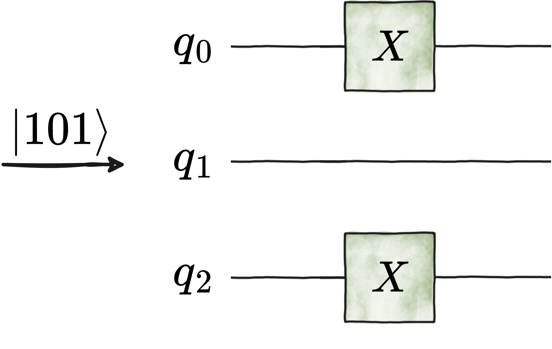
Computational Basis Encoder#
Given a bitstring \(b\) of length \(n\), this encoder generates a layer of Pauli-\(X\) gates that creates the quantum state \(|\,b\,\rangle\).
For instance, the following two circuit generations are equivalent:
b = "101"
circuit_1 = comp_basis_encoder(b)

circuit_2 = Circuit(3)
circuit_2.add(gates.X(0))
circuit_2.add(gates.X(2))
- qibo.models.encodings.comp_basis_encoder(basis_element: int | str | list | tuple, nqubits: int | None = None, **kwargs) Circuit[source]#
Create circuit that performs encoding of bitstrings into computational basis states.
- Parameters:
basis_element (int or str or list or tuple) – bitstring to be encoded. If
int,nqubitsmust be specified. Ifstr, must be composed of only \(0`s and :math:`1`s. If ``list`\) ortuple, must be composed of \(0`s and :math:`1`s as ``int`\) orstr.nqubits (int, optional) – total number of qubits in the circuit. If
basis_elementisint,nqubitsmust be specified. IfnqubitsisNone,nqubitsdefaults to length ofbasis_element. Defaults toNone.kwargs (dict, optional) – Additional arguments used to initialize a Circuit object. For details, see the documentation of
qibo.models.circuit.Circuit.
- Returns:
Circuit encoding computational basis element.
- Return type:
Dicke state#
- qibo.models.encodings.dicke_state(nqubits: int, weight: int, all_to_all: bool = False, **kwargs) Circuit[source]#
Create a circuit that prepares the Dicke state \(\ket{D_{k}^{n}}\).
The Dicke state \(\ket{D_{k}^{n}}\) is the equal superposition of all \(n\)-qubit computational basis states with fixed-Hamming-weight \(k\). The circuit prepares the state deterministically with \(O(k \, n)\) gates and \(O(n)\) depth, or \(O(k \log\frac{n}{k})\) depth under the assumption of
all-to-allconnectivity.- Parameters:
nqubits (int) – number of qubits \(n\).
weight (int) – Hamming weight \(k\) of the Dicke state.
all_to_all (bool, optional) – If
False, uses implementation from Ref. [1]. IfTrue, uses shorter-depth implementation from Ref. [2]. Defaults toFalse.kwargs (dict, optional) – additional arguments used to initialize a Circuit object. For details, see the documentation of
qibo.models.circuit.Circuit.
- Returns:
Circuit that prepares \(\ket{D_{k}^{n}}\).
- Return type:
References
1. Andreas Bärtschi and Stephan Eidenbenz, Deterministic preparation of Dicke states, 22nd International Symposium on Fundamentals of Computation Theory, FCT’19, 126-139 (2019).
2. Andreas Bärtschi and Stephan Eidenbenz, Short-Depth Circuits for Dicke State Preparation, IEEE International Conference on Quantum Computing & Engineering (QCE), 87–96 (2022).
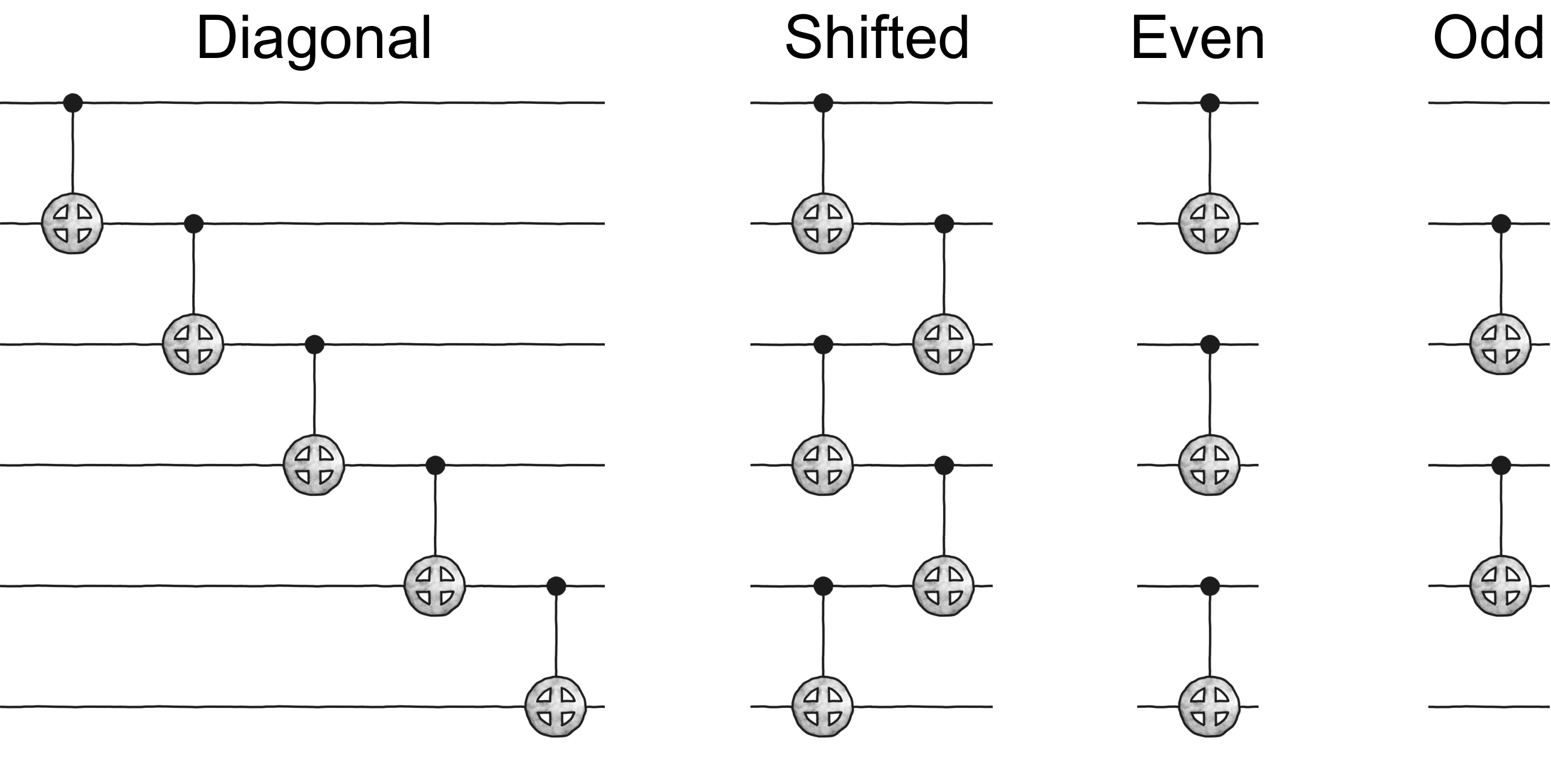
Entangling layer#
Generates a layer of nearest-neighbour two-qubit gates, assuming 1-dimensional connectivity.
With the exception of qibo.gates.gates.GeneralizedfSim,
any of the two-qubit gates implemented in qibo can be selected to customize the entangling layer.
If the chosen gate is parametrized, all phases are set to \(0.0\).
Note that these phases can be updated a posterior by using
qibo.models.Circuit.set_parameters().
The possible choices of layer architecture are the following, in alphabetical order:
diagonal, even_layer, next_nearest, pyramid, odd_layer, shifted, v, and x.
For instance, we show below an example of four of those architectures for nqubits = 6 and entangling_gate = "CNOT".
If closed_boundary is set to True, then an extra gate is added connecting the last and the first qubit,
with the last qubit as the control qubit and the first qubit as a target qubit.
- qibo.models.encodings.entangling_layer(nqubits: int, architecture: str = 'diagonal', entangling_gate: str | Gate = 'CNOT', closed_boundary: bool = False, **kwargs) Circuit[source]#
Create a layer of two-qubit entangling gates.
If the chosen gate is a parametrized gate, all phases are set to \(0.0\).
- Parameters:
nqubits (int) – Total number of qubits in the circuit.
architecture (str, optional) – Architecture of the entangling layer. In alphabetical order, options are
"diagonal","even_layer","next_nearest","odd_layer","pyramid","shifted","v", and"x". The"x"architecture is only defined for an even number of qubits. Defaults to"diagonal".entangling_gate (str or
qibo.gates.Gate, optional) – Two-qubit gate to be used in the entangling layer. Ifentangling_gateis a parametrized gate, all phases are initialized as \(0.0\). Defaults to"CNOT".closed_boundary (bool, optional) – If
Trueandarchitecture not in ["pyramid", "v", "x"], adds a closed-boundary condition to the entangling layer. Defaults toFalse.kwargs (dict, optional) – Additional arguments used to initialize a Circuit object. For details, see the documentation of
qibo.models.circuit.Circuit.
- Returns:
Circuit containing layer of two-qubit gates.
- Return type:
Greenberger-Horne-Zeilinger (GHZ) state#
- qibo.models.encodings.ghz_state(nqubits: int, **kwargs) Circuit[source]#
Generate an \(n\)-qubit Greenberger-Horne-Zeilinger (GHZ) state that takes the form
\[\ket{\text{GHZ}} = \frac{\ket{0}^{\otimes n} + \ket{1}^{\otimes n}}{\sqrt{2}}\]where \(n\) is the number of qubits.
- Parameters:
nqubits (int) – number of qubits \(n >= 2\).
kwargs (dict, optional) – additional arguments used to initialize a Circuit object. For details, see the documentation of
qibo.models.circuit.Circuit.
- Returns:
Circuit that prepares the GHZ state.
- Return type:
Graph state#
- qibo.models.encodings.graph_state(matrix: _Buffer | _SupportsArray[dtype[Any]] | _NestedSequence[_SupportsArray[dtype[Any]]] | bool | int | float | complex | str | bytes | _NestedSequence[bool | int | float | complex | str | bytes], backend: Backend | None = None, **kwargs) Circuit[source]#
Create circuit encoding an undirected graph state given its adjacency matrix.
Given a graph \(G = (V, E)\) with \(V\) being the set of vertices and \(E\) being the set of edges, an $n$-qubit graph state is defined as
\[\ket{G} = \prod_{(j, k) \in E} \, CZ_{j, k} \, \ket{+}^{\otimes V} \, ,\]where \(CZ_{a,b}\) is the
qibo.gates.CZgate acting on qubits \(j\) and \(k\), and \(\ket{+} = H \, \ket{0}$, with :class:`qibo.gates.H\) being the Hadamard gate.- Parameters:
matrix (ArrayLike or list) – Adjacency matrix of the graph.
backend (
qibo.backends.abstract.Backend, optional) – backend to be used in the execution. IfNone, it uses the current backend. Defaults toNone.kwargs (dict, optional) – Additional arguments used to initialize a Circuit object. For details, see the documentation of
qibo.models.circuit.Circuit.
- Returns:
Circuit of the graph state with the given adjacency matrix.
- Return type:
Fixed Hamming-weight Encoder#
- qibo.models.encodings.hamming_weight_encoder(nqubits: int, weight: int, data: _Buffer | _SupportsArray[dtype[Any]] | _NestedSequence[_SupportsArray[dtype[Any]]] | bool | int | float | complex | str | bytes | _NestedSequence[bool | int | float | complex | str | bytes] | None = None, complex_data: bool = False, full_hwp: bool = False, optimize_controls: bool = True, phase_correction: bool = True, initial_string: _Buffer | _SupportsArray[dtype[Any]] | _NestedSequence[_SupportsArray[dtype[Any]]] | bool | int | float | complex | str | bytes | _NestedSequence[bool | int | float | complex | str | bytes] | None = None, backend: Backend | None = None, **kwargs) Circuit[source]#
Create circuit that encodes
datain the Hamming-weight-\(k\) basis ofnqubits.Let \(\mathbf{x}\) be a \(1\)-dimensional array of size \(d = \binom{n}{k}\) and \(B_{k} \equiv \{ \ket{b_{j}} : b_{j} \in \{0, 1\}^{\otimes n} \,\, \text{and} \,\, |b_{j}| = k \}\) be a set of \(d\) computational basis states of \(n\) qubits that are represented by bitstrings of Hamming weight \(k\). Then, an amplitude encoder in the basis \(B_{k}\) is an \(n\)-qubit parameterized quantum circuit \(\operatorname{Load}_{B_{k}}\) such that
\[\operatorname{Load}(\mathbf{x}) \, \ket{0}^{\otimes n} = \frac{1}{\|\mathbf{x}\|} \, \sum_{j = 1}^{d} \, x_{j} \, \ket{b_{j}}\]- Parameters:
nqubits (int) – number of qubits.
weight (int) – Hamming weight that defines the subspace in which
datawill be encoded.data (ArrayLike, optional) – \(1\)-dimensional array of data to be loaded. If
None, circuit is returned with all phases set to \(0.0\). Defaults toNone.complex_data (bool, optional) – to be used when
data is None. IfTrue, returned circuit parametrizes complex-valued states. IfFalse, it parametrizes real-valued states. Ifdata is not None, then data type is inferred fromdata. Defaults toFalse.full_hwp (bool, optional) – if
False, includes Pauli-\(X\) gates that prepare the first bitstring of Hamming weightk = weight. IfTrue, circuit is full Hamming weight preserving. Defaults to`False.optimize_controls (bool, optional) – if
True, removes unnecessary controlled operations. Defaults toTrue.phase_correction (bool, optional) – To be used when
datais complex-valued. IfTrue, adds a controlled-$mathrm{RZ}$ gate to the end of the circuit, adding a final phase correction. IfFalse, gate is not added. Defaults toTrue.initial_string (ArrayLike, optional) – Array containing the desired initial bitstring of Hamming
weight$k$. IfNone, defaults to $ket{1^{k}0^{n-k}}$. Defaults toNone.backend (
qibo.backends.abstract.Backend, optional) – backend to be used in the execution. IfNone, it uses the current backend. Defaults toNone.kwargs (dict, optional) – Additional arguments used to initialize a Circuit object. For details, see the documentation of
qibo.models.circuit.Circuit.
- Returns:
Circuit that loads
datain Hamming-weight-\(k\) representation.- Return type:
References
1. R. M. S. Farias, T. O. Maciel, G. Camilo, R. Lin, S. Ramos-Calderer, and L. Aolita, Quantum encoder for fixed-Hamming-weight subspaces Phys. Rev. Applied 23, 044014 (2025).
Permutation synthesis#
- qibo.models.encodings.permutation_synthesis(sigma: List[int] | tuple[int, ...], m: int = 2, backend: Backend | None = None, **kwargs) Circuit[source]#
Return circuit that implements a given permutation.
Given permutation
sigmaon \(\{0, \, 1, \, \dots, \, d-1\}\) and a power‑of‑two budgetm, this function factorssigmainto the fewest layers \(\sigma_{1}, \, \sigma_{2}, \, \cdots, \, \sigma_{t}\) such that:each layer has at most \(m\) disjoint transpositions;
each layer moves a power‑of‑two number of indices.
The function returns a circuit synthesis of
sigma.- Parameters:
sigma (list or tuple) – permutation description on \(\{0, \, 1, \, \dots, \, d-1\}\).
m (int) – power‑of‑two budget. Defauls to \(2\).
backend (
qibo.backends.abstract.Backend, optional) – backend to be used in the execution. IfNone, it uses the current backend. Defaults toNone.kwargs (dict, optional) – Additional arguments used to initialize a Circuit object. For details, see the documentation of
qibo.models.circuit.Circuit.
- Returns:
Circuit that implements the permutation
sigma.- Return type:
References
1. L. Li, and J. Luo, Nearly Optimal Circuit Size for Sparse Quantum State Preparation arXiv:2406.16142 (2024).
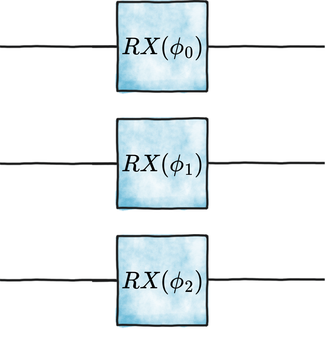
Phase Encoder#
Encodes data of length \(n\) into the phases of \(n\) qubits.
For instance, the following two circuit generations are equivalent:
nqubits = 3
phases = np.random.rand(nqubits)

circuit_1 = phase_encoder(nqubits, rotation="RX", data=phases)

circuit_2 = Circuit(3)
circuit_2.add(gates.RX(qubit, phases[qubit]) for qubit in range(nqubits))
- qibo.models.encodings.phase_encoder(nqubits: int, rotation: str = 'RY', data: _Buffer | _SupportsArray[dtype[Any]] | _NestedSequence[_SupportsArray[dtype[Any]]] | bool | int | float | complex | str | bytes | _NestedSequence[bool | int | float | complex | str | bytes] | None = None, backend: Backend | None = None, **kwargs) Circuit[source]#
Create circuit that performs the phase encoding of
data.- Parameters:
nqubits (int) – number of qubits in the system.
rotation (str, optional) – If
"RX", usesqibo.gates.gates.RXas rotation. If"RY", usesqibo.gates.gates.RYas rotation. If"RZ", usesqibo.gates.gates.RZas rotation. Defaults to"RY".data (ArrayLike) – \(1\)-dimensional array of phases to be loaded. If
None, all phases of the circuit are set to \(0.0\). Defaults toNone.backend (
qibo.backends.abstract.Backend, optional) – backend to be used in the execution. IfNone, it uses the current backend. Defaults toNone.kwargs (dict, optional) – Additional arguments used to initialize a Circuit object. For details, see the documentation of
qibo.models.circuit.Circuit.
- Returns:
Circuit that loads
datain phase encoding.- Return type:
Sparse encoder#
- qibo.models.encodings.sparse_encoder(data: _Buffer | _SupportsArray[dtype[Any]] | _NestedSequence[_SupportsArray[dtype[Any]]] | bool | int | float | complex | str | bytes | _NestedSequence[bool | int | float | complex | str | bytes], method: str = 'li', nqubits: int | None = None, backend: Backend | None = None, **kwargs) Circuit[source]#
Create circuit that encodes \(1\)-dimensional data in a subset of amplitudes of the computational basis.
Consider a sparse-access model, where for a data vector \(\mathbf{x} \in \mathbb{C}^{d}\), with \(d = 2^{n}\) and \(s\) non-zero amplitudes, one has access to the data vector \(\mathbf{y}\) of the form
\[\mathbf{y} = \left\{ (b_{1}, x_{1}), \, \dots, \, (b_{s}, x_{s}) \right\} \, ,\]where \(\{x_{j}\}_{j\in[s]}\) is the non-zero components of \(\mathbf{x}\) and \(\{b_{j}\}_{j\in[s]}\) is the set of addresses associated with these values. Then, this function generates a quantum circuit \(s\text{-}\mathrm{Load}\) that encodes \(\mathbf{x}\) in the amplitudes of an \(n\)-qubit quantum state as
\[s\text{-}\mathrm{Load}(\mathbf{y}) \, \ket{0}^{\otimes \, n} = \sum_{j\in[s]} \, \frac{x_{j}}{\|\mathbf{x}\|_{2}} \, \ket{b_{j}} \, ,\]where \(\|\cdot\|_{2}\) is the Euclidean norm.
The resulting circuit parametrizes
datain hyperspherical coordinates in the \((2^{n} - 1)\)-unit sphere.- Parameters:
data (ArrayLike or list or zip) – sequence of tuples of the form \((b_{j}, x_{j})\). The addresses \(b_{j}\) can be either integers or in bitstring format of size \(n\).
method (str, optional) – method to be used, either
liorfarias. They refer to methods in references [1] and [2], respectively. Defaults tolinqubits (int, optional) – total number of qubits in the system. To be used when \(b_j\) are integers. If \(b_j\) are strings and
nqubitsisNone, defaults to the length of the strings \(b_{j}\). Defaults toNone.backend (
qibo.backends.abstract.Backend, optional) – backend to be used in the execution. IfNone, it uses the current backend. Defaults toNone.kwargs (dict, optional) – Additional arguments used to initialize a Circuit object. For details, see the documentation of
qibo.models.circuit.Circuit.
- Returns:
Circuit that loads sparse \(\mathbf{x}\).
- Return type:
References
1. L. Li, and J. Luo, Nearly optimal circuit size for sparse quantum state preparation arXiv:2406.16142 (2024).
2. R. M. S. Farias, T. O. Maciel, G. Camilo, R. Lin, S. Ramos-Calderer, and L. Aolita, Quantum encoder for fixed-Hamming-weight subspaces, Phys. Rev. Applied 23, 044014 (2025).
Unary Encoder#
Given a classical data array \(\mathbf{x} \in \mathbb{R}^{d}\) such that
this function generate the circuit that prepares the following quantum state \(\ket{\psi} \in \mathcal{H}\):
with \(\mathcal{H} \cong \mathbb{C}^{d}\) being a \(d\)-qubit Hilbert space, and \(\|\cdot\|_{\textup{HS}}\) being the Hilbert-Schmidt norm.
Here, \(\ket{k}\) is a unary representation of the number \(k\). For instance, for \(d = 3\), the final state would be
There are multiple circuit architechtures that lead to unary encoding of classical data. For example, to encode a \(8\)-dimensional data, one could use the so-called tree architechture below:
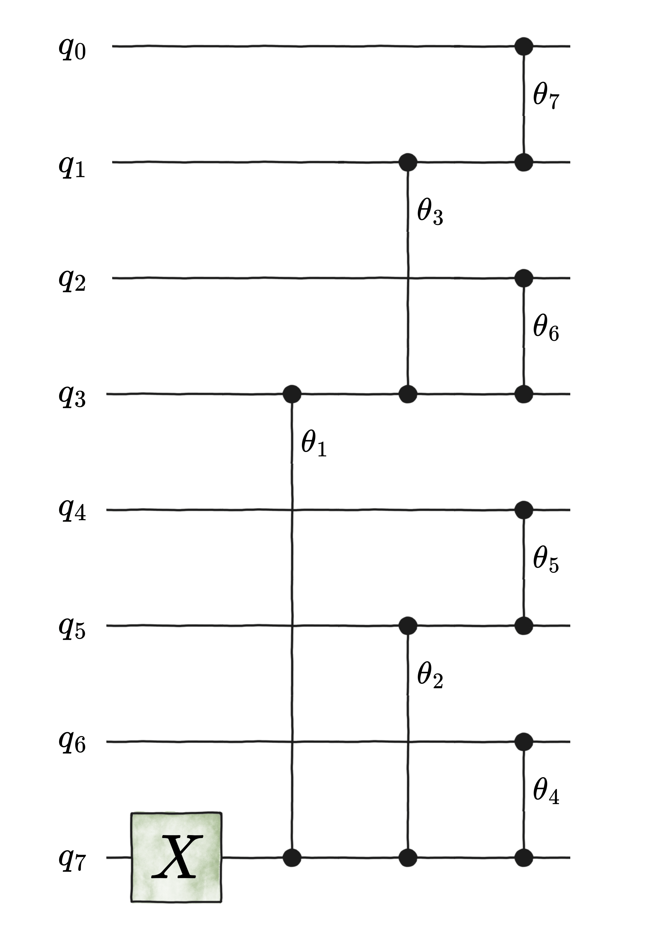
where the first gate is the qibo.gates.X
and the parametrized gates are the qibo.gates.RBS.
To know how the angles \(\{\theta_{k}\}_{[k]}\) are calculated for this architecture,
please refer to S. Johri et al., Nearest Centroid Classification on a Trapped Ion Quantum Computer,
arXiv:2012.04145v2 [quant-ph].
On the other hand, the same encoding could be performed using the so-called diagonal (also known as ladder) architecture below:
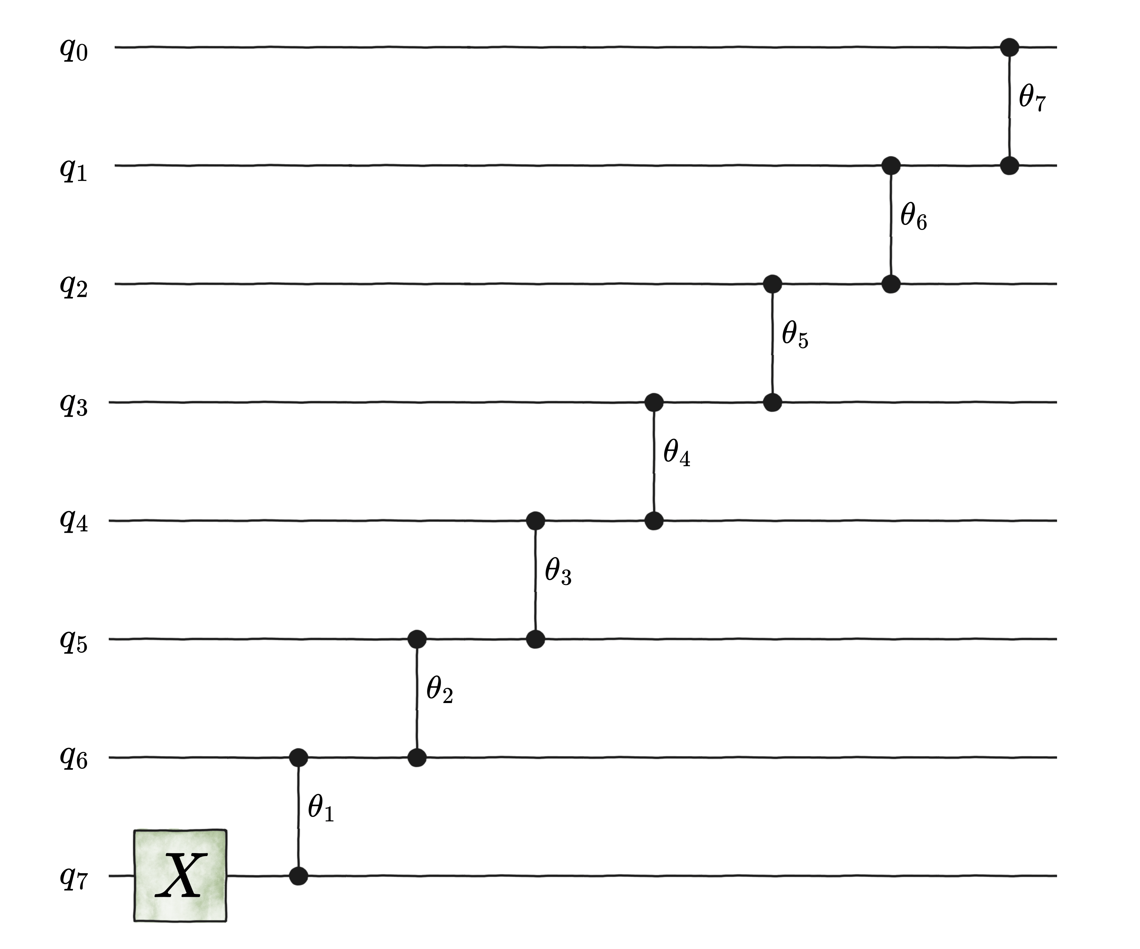
This architecture leads to a choice of angles based on spherical coordinates in a d-dimensional hypersphere.
- qibo.models.encodings.unary_encoder(nqubits: int, architecture: str = 'tree', data: _Buffer | _SupportsArray[dtype[Any]] | _NestedSequence[_SupportsArray[dtype[Any]]] | bool | int | float | complex | str | bytes | _NestedSequence[bool | int | float | complex | str | bytes] | None = None, backend: Backend | None = None, **kwargs) Circuit[source]#
Create circuit that performs the (deterministic) unary encoding of
data.- Parameters:
nqubits (int) – number of qubits in the system.
architecture (str, optional) – circuit architecture used for the unary loader. If
diagonal, uses a ladder-like structure. Iftree, uses a binary-tree-based structure. Defaults totree.data (ArrayLike) – \(1\)-dimensional array of data to be loaded. If
None, all phases in the returned circuit are set to \(0.0\).backend (
qibo.backends.abstract.Backend, optional) – backend to be used in the execution. IfNone, it uses the current backend. Defaults toNone.kwargs (dict, optional) – Additional arguments used to initialize a Circuit object. For details, see the documentation of
qibo.models.circuit.Circuit.
- Returns:
Circuit that loads
datain unary representation.- Return type:
Unary Encoder for Random Gaussian States#
Performs the same unary encoder as qibo.models.encodings.unary_encoder
using the tree architecture , with the difference being that now each entry
of the \(d\)-dimensional array is sampled from a Gaussian distribution
\(\mathcal{N}(0, 1)\).
- qibo.models.encodings.unary_encoder_random_gaussian(nqubits: int, architecture: str = 'tree', seed: int | None = None, backend: Backend | None = None, **kwargs) Circuit[source]#
Create a circuit that performs the unary encoding of a random Gaussian state.
At depth \(h\) of the tree architecture, the angles \(\theta_{k} \in [0, 2\pi]\) of the the gates \(RBS(\theta_{k})\) are sampled from the following probability density function:
\[p_{h}(\theta) = \frac{1}{2} \, \frac{\Gamma(2^{h-1})}{\Gamma^{2}(2^{h-2})} \, \left|\sin(\theta) \, \cos(\theta)\right|^{2^{h-1} - 1} \, ,\]where \(\Gamma(\cdot)\) is the Gamma function.
- Parameters:
nqubits (int) – number of qubits.
architecture (str, optional) – circuit architecture used for the unary loader. If
tree, uses a binary-tree-based structure. Defaults totree.seed (int or
numpy.random.Generator, optional) – Either a generator of random numbers or a fixed seed to initialize a generator. IfNone, initializes a generator with a random seed. Defaults toNone.backend (
qibo.backends.abstract.Backend, optional) – backend to be used in the execution. IfNone, it uses the current backend. Defaults toNone.kwargs (dict, optional) – Additional arguments used to initialize a Circuit object. For details, see the documentation of
qibo.models.circuit.Circuit.
- Returns:
Circuit that loads a random Gaussian array in unary representation.
- Return type:
References
1. A. Bouland, A. Dandapani, and A. Prakash, A quantum spectral method for simulating stochastic processes, with applications to Monte Carlo. arXiv:2303.06719v1 [quant-ph]
Up-to-Hamming-weight-\(k\) Encoder#
- qibo.models.encodings.up_to_k_hamming_weight_encoder(nqubits: int, up_to_k: int, data: _Buffer | _SupportsArray[dtype[Any]] | _NestedSequence[_SupportsArray[dtype[Any]]] | bool | int | float | complex | str | bytes | _NestedSequence[bool | int | float | complex | str | bytes] | None = None, complex_data: bool = False, codewords: List[int] | None = None, keep_antictrls: bool = False, backend: Backend | None = None, **kwargs) Circuit[source]#
Create a circuit that encodes
datain the Hamming-weight-\(\leq k\) subspace ofnqubits.Let \(\mathbf{x}\) be a \(1\)-dimensional array of size
\[d = \sum_{l=0}^{k} \binom{n}{l},\]and define the union-Hamming-weight-subspace
\[B_{\le k} \equiv \left\{ \ket{b_j} : b_j \in \{0,1\}^{\otimes n}, \; |b_j| \le k \right\},\]i.e., the set of all computational basis states of \(n\) qubits whose bitstrings have Hamming weight less than or equal to \(k\). Equivalently,
\[B_{\le k} = \bigcup_{w=0}^{k} B_w,\]where \(B_w\) denotes the set of basis states of fixed Hamming weight \(w\).
An amplitude encoder in the basis \(B_{\le k}\) is an \(n\)-qubit parameterized quantum circuit \(\operatorname{Load}_{B_{\le k}}\) such that
\[\operatorname{Load}_{B_{\le k}}(\mathbf{x}) \, \ket{0}^{\otimes n} = \frac{1}{\|\mathbf{x}\|} \sum_{j=1}^{d} x_j \ket{b_j},\]where \(\{ \ket{b_j} \}_{j=1}^d\) is an enumeration of the elements of \(B_{\le k}\).
Resulting circuit parametrizes
datain eitherhypersphericalorhopfcoordinates in the \((2^{n} - 1)\)-unit sphere.- Parameters:
nqubits (int) – total number of qubits in the system.
up_to_k (int) – upper limit for the Hamming weight of the union-Hamming-weight-subspace in which the data to be loaded will be supported.
data (ArrayLike, optional) – \(1\)-dimensional array of length \(d = \sum_{l=0}^{k} \binom{n}{l}\) to be loaded in the amplitudes of a \(n\)-qubit quantum state. If
None, all phases of the returned circuit are set to \(0.0\). Defaults toNone.complex_data (bool, optional) – to be used when
data is None. IfTrue, returned circuit parametrizes complex-valued states. IfFalse, it parametrizes real-valued states. Ifdata is not None, then data type is inferred fromdata. Defaults toFalse.codewords (list, optional) – List of codewords used to encode the data in the given order. If
None, the codewords are set by the erhlich algorithm.keep_antictrls (bool, optional) – If
Trueand parametrization ishyperspherical, we don’t simplify the anti-controls when placing the RBS gates. For details, see [1].backend (
qibo.backends.abstract.Backend, optional) – backend to be used in the execution. IfNone, it uses the current backend. Defaults toNone.kwargs (dict, optional) – Additional arguments used to initialize a Circuit object. For details, see the documentation of
qibo.models.circuit.Circuit.
- Returns:
Circuit that loads
datain up-to-k encoding.- Return type:
References
1. R. M. S. Farias, T. O. Maciel, G. Camilo, R. Lin, S. Ramos-Calderer, and L. Aolita, Quantum encoder for fixed-Hamming-weight subspaces Phys. Rev. Applied 23, 044014 (2025).
Error Mitigation#
Qibo allows for mitigating noise in circuits via error mitigation methods. Unlike error correction, error mitigation does not aim to correct qubit errors, but rather it provides the means to estimate the noise-free expected value of an observable measured at the end of a noisy circuit.
Readout Mitigation#
A common kind of error happening in quantum circuits is readout error, i.e. the error in the measurement of the qubits at the end of the computation. In Qibo there are currently two methods implemented for mitigating readout errors, and both can be used as standalone functions or in combination with the other general mitigation methods by setting the paramter readout.
Response Matrix#
Given \(n\) qubits, all the possible \(2^n\) states are constructed via the application of the corresponding sequence of \(X\) gates \(X_0\otimes I_1\otimes\cdot\cdot\cdot\otimes X_{n-1}\). In the presence of readout errors, we will measure for each state \(i\) some noisy frequencies \(F_i^{noisy}\) different from the ideal ones \(F_i^{ideal}=\delta_{i,j}\).
The effect of the error is modeled by the response matrix composed of the noisy frequencies as columns \(M=\big(F_0^{noisy},...,F_{n-1}^{noisy}\big)\). We have indeed that:
and, therefore, the calibration matrix obtained as \(M_{\text{cal}}=M^{-1}\) can be used to recover the noise-free frequencies.
The calibration matrix \(M_{\text{cal}}\) lacks stochasticity, resulting in a ‘negative probability’ issue. The distributions that arise after applying \(M_{\text{cal}}\) are quasiprobabilities; the individual elements can be negative surpass 1, provided they sum to 1. It is posible to use Iterative Bayesian Unfolding (IBU) to preserve non-negativity. See Nachman et al for more details.
- qibo.models.error_mitigation.get_response_matrix(nqubits: int, qubit_map: List[int] | None = None, noise_model: NoiseModel | None = None, nshots: int = 10000, backend: Backend | None = None)[source]#
Computes the response matrix for readout mitigation.
- Parameters:
nqubits (int) – Total number of qubits.
qubit_map (list, optional) – the qubit map. If None, a list of range of circuit’s qubits is used. Defaults to
None.noise_model (
qibo.noise.NoiseModel, optional) – noise model used for simulating noisy computation. This matrix can be used to mitigate the effect of qibo.noise.ReadoutError.nshots (int, optional) – number of shots. Defaults to \(10000\).
backend (
qibo.backends.abstract.Backend, optional) – backend to be used in the execution. IfNone, it uses the current backend. Defaults toNone.
- Returns:
the computed (nqubits, nqubits) response matrix for readout mitigation.
- Return type:
ArrayLike
- qibo.models.error_mitigation.iterative_bayesian_unfolding(probabilities: _Buffer | _SupportsArray[dtype[Any]] | _NestedSequence[_SupportsArray[dtype[Any]]] | bool | int | float | complex | str | bytes | _NestedSequence[bool | int | float | complex | str | bytes], response_matrix: _Buffer | _SupportsArray[dtype[Any]] | _NestedSequence[_SupportsArray[dtype[Any]]] | bool | int | float | complex | str | bytes | _NestedSequence[bool | int | float | complex | str | bytes], iterations: int = 10)[source]#
Iterative Bayesian Unfolding (IBU) method for readout mitigation.
- Parameters:
probabilities (ArrayLike) – the input probabilities to be unfolded.
response_matrix (ArrayLike) – the response matrix.
iterations (int, optional) – the number of iterations to perform. Defaults to 10.
- Returns:
the unfolded probabilities.
- Return type:
ArrayLike
- Reference:
1. B. Nachman, M. Urbanek et al, Unfolding Quantum Computer Readout Noise. arXiv:1910.01969 [quant-ph]. 2. S. Srinivasan, B. Pokharel et al, Scalable Measurement Error Mitigation via Iterative Bayesian Unfolding. arXiv:2210.12284 [quant-ph].
- qibo.models.error_mitigation.apply_resp_mat_readout_mitigation(state: CircuitResult, response_matrix: _Buffer | _SupportsArray[dtype[Any]] | _NestedSequence[_SupportsArray[dtype[Any]]] | bool | int | float | complex | str | bytes | _NestedSequence[bool | int | float | complex | str | bytes], iterations: int | None = None)[source]#
Applies readout error mitigation to the given state using the provided response matrix.
- Parameters:
state (
qibo.measurements.CircuitResult) – the input state to be updated. This state should contain the frequencies that need to be mitigated.response_matrix (numpy.ndarray) – the response matrix for readout mitigation.
iterations (int, optional) – the number of iterations to use for the Iterative Bayesian Unfolding method. If
Nonethe ‘inverse’ method is used. Defaults toNone.
- Returns:
the input state with the updated (mitigated) frequencies.
- Return type:
qibo.measurements.CircuitResult
- qibo.models.error_mitigation.apply_randomized_readout_mitigation(circuit, noise_model=None, nshots: int = 10000, ncircuits: int = 10, qubit_map=None, seed: int | None = None, backend=None)[source]#
Readout mitigation method that transforms the bias in an expectation value into a measurable multiplicative factor.
This factor can be eliminated at the expense of increased sampling complexity for the observable.
- Parameters:
circuit (
qibo.models.Circuit) – input circuit.noise_model (
qibo.noise.NoiseModel, optional) – noise model used for simulating noisy computation. Defaults toNone.nshots (int, optional) – number of shots. Defaults to \(10000\).
ncircuits (int, optional) – number of randomized circuits. Each of them uses
int(nshots / ncircuits)shots. Defaults to 10.qubit_map (list, optional) – the qubit map. If
None, a list of range of circuit’s qubits is used. Defaults toNone.seed (int or
numpy.random.Generator, optional) – Either a generator of random numbers or a fixed seed to initialize a generator. IfNone, initializes a generator with a random seed. Default:None.backend (
qibo.backends.abstract.Backend, optional) – backend to be used in the execution. IfNone, it uses the current backend. Defaults toNone.
- Returns:
- the state of the input circuit with
mitigated frequencies.
- Return type:
qibo.measurements.CircuitResult
References
1. Ewout van den Berg, Zlatko K. Minev et al, Model-free readout-error mitigation for quantum expectation values. arXiv:2012.09738 [quant-ph].
- qibo.models.error_mitigation.get_expectation_val_with_readout_mitigation(circuit: Circuit, observable: Hamiltonian | SymbolicHamiltonian, noise_model: NoiseModel | None = None, nshots: int = 10000, readout: dict | None = None, qubit_map: List[int] | None = None, seed: int | None = None, backend: Backend | None = None)[source]#
CDR: Applies readout error mitigation to the given circuit and observable.
- Parameters:
circuit (
qibo.models.Circuit) – input circuit.observable (
qibo.hamiltonians.Hamiltonian/:class:`qibo.hamiltonians.SymbolicHamiltonian) – The observable to be measured.noise_model (
qibo.models.noise.NoiseModel, optional) – the noise model to be applied. Defaults toNone.nshots (int, optional) – the number of shots for the circuit execution. Defaults to \(10^{4}\).
readout (dict, optional) –
a dictionary that may contain the following keys: * ncircuits: int, specifies the number of random circuits to use for the
randomized method of readout error mitigation.
response_matrix: numpy.ndarray, used for applying a pre-computed response matrix for readout error mitigation.
ibu_iters: int, specifies the number of iterations for the iterative Bayesian unfolding method of readout error mitigation. If provided, the corresponding readout error mitigation method is used. Defaults to an empty
dict.
qubit_map (list, optional) – the qubit map. If None, a list of range of circuit’s qubits is used. Defaults to
None.seed (int or
numpy.random.Generator, optional) – Either a generator of random numbers or a fixed seed to initialize a generator. IfNone, initializes a generator with a random seed. Default:None.backend (qibo.backends.abstract.Backend, optional) – the backend to be used in the execution. If
None, it uses the global backend. Defaults toNone.
- Returns:
The mitigated expectation value of the observable.
- Return type:
Randomized readout mitigation#
This approach converts the effect of any noise map \(A\) into a single multiplication factor for each Pauli observable, that is, diagonalizes the measurement channel. The multiplication factor \(\lambda\) can be directly measured even without the quantum circuit. Dividing the measured value \(\langle O\rangle_{noisy}\) by these factor results in the mitigated Pauli expectation value \(\langle O\rangle_{ideal}\),
This process can be implemented with the aforementioned
qibo.models.error_mitigation.apply_randomized_readout_mitigation().
Zero Noise Extrapolation (ZNE)#
Given a noisy circuit \(C\) and an observable \(A\), Zero Noise Extrapolation (ZNE) consists in running \(n+1\) versions of the circuit with different noise levels \(\{c_j\}_{j=0..n}\) and, for each of them, measuring the expected value of the observable \(E_j=\langle A\rangle_j\).
Then, an estimate for the expected value of the observable in the noise-free condition is obtained as:
with \(\gamma_j\) satisfying:
This implementation of ZNE relies on the insertion of gate pairs (that resolve to the identity in the noise-free case) to realize the different noise levels \(\{c_j\}\), see He et al for more details. Hence, the canonical levels are mapped to the number of inserted pairs as \(c_j\rightarrow 2 c_j + 1\).
- qibo.models.error_mitigation.ZNE(circuit: Circuit, observable: Hamiltonian | SymbolicHamiltonian, noise_levels: _Buffer | _SupportsArray[dtype[Any]] | _NestedSequence[_SupportsArray[dtype[Any]]] | bool | int | float | complex | str | bytes | _NestedSequence[bool | int | float | complex | str | bytes], noise_model: NoiseModel = None, nshots: int = 10000, solve_for_gammas: bool = False, global_unitary_folding: bool = True, insertion_gate: str = 'CNOT', readout: dict = None, qubit_map: List[int] = None, seed: int | None = None, backend: Backend | None = None)[source]#
Runs the Zero Noise Extrapolation (ZNE) method for error mitigation.
The different noise levels are realized by the insertion of pairs of either
CNOTorRX(pi/2)gates that resolve to the identiy in the noise-free case.- Parameters:
circuit (
qibo.models.Circuit) – input circuit.observable (
qibo.hamiltonians.Hamiltonianorqibo.hamiltonians.SymbolicHamiltonian) – Observable to measure.noise_levels (ndarray) – Sequence of noise levels.
noise_model (
qibo.noise.NoiseModel, optional) – Noise model applied to simulate noisy computation.nshots (int, optional) – Number of shots. Defaults to \(10000\). If
None, the circuit is simulated without sampling: with statevector simulation if noise_model is not None and with density matrix simulation otherwise. Readout mitigation is not available with exact simulation.solve_for_gammas (bool, optional) – If
True, explicitly solve the equations to obtain thegammacoefficients. Default isFalse.global_unitary_folding (bool, optional) – If
True, noise is increased by global unitary folding. IfFalse, local unitary folding is used. Defaults toTrue.insertion_gate (str, optional) – gate to be folded in the local unitary folding. If
RX, the gate used is :math:RX(\pi / 2). Otherwise, it is theqibo.gates.gates.CNOTgate.readout (dict, optional) –
a dictionary that may contain the following keys: * ncircuits: int, specifies the number of random circuits to use for the
randomized method of readout error mitigation.
response_matrix:
ndarray, used for applying a pre-computed response matrix for readout error mitigation.ibu_iters: int, specifies the number of iterations for the iterative Bayesian unfolding method of readout error mitigation. If provided, the corresponding readout error mitigation method is used. Defaults to an empty
dict.
qubit_map (list, optional) – the qubit map. If None, a list of range of circuit’s qubits is used. Defaults to
None.seed (int or
numpy.random.Generator, optional) – Either a generator of random numbers or a fixed seed to initialize a generator. IfNone, initializes a generator with a random seed. Default:None.backend (
qibo.backends.abstract.Backend, optional) – backend to be used in the execution. IfNone, it uses the current backend. Defaults toNone.
- Returns:
Estimate of the expected value of
observablein the noise free condition.- Return type:
ArrayLike
- Reference:
1. K. Temme, S. Bravyi et al, Error mitigation for short-depth quantum circuits. Phys. Rev. Lett. 119, 180509 (2017).
- qibo.models.error_mitigation.get_gammas(noise_levels: _Buffer | _SupportsArray[dtype[Any]] | _NestedSequence[_SupportsArray[dtype[Any]]] | bool | int | float | complex | str | bytes | _NestedSequence[bool | int | float | complex | str | bytes], analytical: bool = True)[source]#
Standalone function to compute the ZNE coefficients given the noise levels.
- Parameters:
noise_levels (numpy.ndarray) – array containing the different noise levels. Note that in the CNOT insertion paradigm this corresponds to the number of CNOT pairs to be inserted. The canonical ZNE noise levels are obtained as
2 * c + 1.analytical (bool, optional) – if
True, computes the coeffients by solving the linear system. IfFalse, use the analytical solution valid for the CNOT insertion method. Default isTrue.
- Returns:
the computed coefficients.
- Return type:
numpy.ndarray
- qibo.models.error_mitigation.get_noisy_circuit(circuit: Circuit, num_insertions: int, global_unitary_folding: bool = True, insertion_gate: bool = None)[source]#
Standalone function to generate the noisy circuit with the inverse gate pairs insertions.
- Parameters:
circuit (
qibo.models.circuit.Circuit) – circuit to modify.num_insertions (int) – number of insertion gate pairs / global unitary folds to add.
global_unitary_folding (bool) – If
True, noise is increased by global unitary folding. IfFalse, local unitary folding is used. Defaults toTrue.insertion_gate (str, optional) – gate to be folded in the local unitary folding. If
RX, the gate used is :math:RX(\pi / 2). Otherwise, it is theCNOTgate.
- Returns:
circuit with the inserted gate pairs or with global folding.
- Return type:
qibo.models.Circuit
Clifford Data Regression (CDR)#
In the Clifford Data Regression (CDR) method, a set of \(n\) circuits \(S_n=\{C_i\}_{i=1,..,n}\) is generated starting from the original circuit \(C_0\) by replacing some of the non-Clifford gates with Clifford ones. Given an observable \(A\), all the circuits of \(S_n\) are both simulated to obtain the correspondent expected values of \(A\) in noise-free condition \(\{a_i^{exact}\}_{i=1,..,n}\), and run in noisy conditions to obtain the noisy expected values \(\{a_i^{noisy}\}_{i=1,..,n}\).
Finally a model \(f\) is trained to minimize the mean squared error:
and learn the mapping \(a^{noisy}\rightarrow a^{exact}\). The mitigated expected value of \(A\) at the end of \(C_0\) is then obtained simply with \(f(a_0^{noisy})\).
In this implementation the initial circuit is expected to be decomposed in the three Clifford gates \(RX(\frac{\pi}{2})\), \(CNOT\), \(X\) and in \(RZ(\theta)\) (which is Clifford only for \(\theta=\frac{n\pi}{2}\)). By default the set of Clifford gates used for substitution is \(\{RZ(0),RZ(\frac{\pi}{2}),RZ(\pi),RZ(\frac{3}{2}\pi)\}\). See Sopena et al for more details.
- qibo.models.error_mitigation.CDR(circuit: Circuit, observable: ~qibo.hamiltonians.hamiltonians.Hamiltonian | ~qibo.hamiltonians.hamiltonians.SymbolicHamiltonian, noise_model: ~qibo.noise.NoiseModel, nshots: int = 10000, model: callable = <function <lambda>>, n_training_samples: int = 100, full_output: bool = False, readout: dict | None = None, qubit_map: ~typing.List[int] | None = None, seed: int | None = None, backend: ~qibo.backends.abstract.Backend | None = None)[source]#
Runs the Clifford Data Regression error mitigation method.
- Parameters:
circuit (
qibo.models.Circuit) – input circuit decomposed in the primitive gatesX,CNOT,RX(pi/2),RZ(theta).observable (
qibo.hamiltonians.Hamiltonian/:class:`qibo.hamiltonians.SymbolicHamiltonian) – observable to be measured.noise_model (
qibo.noise.NoiseModel) – noise model used for simulating noisy computation.nshots (int, optional) – Number of shots. Defaults to \(10000\). If None, the circuit is simulated without sampling: with statevector simulation if noise_model is not None and with density matrix simulation otherwise. Readout mitigation is not available with exact simulation.
model (callable, optional) – model used for fitting. This should be a callable function object
f(x, *params), taking as input the predictor variable and the parameters. Default is a simple linear modelf(x,a,b) := a*x + b.n_training_samples (int, optional) – number of training circuits to sample. Defaults to \(100\).
full_output (bool, optional) – if
True, this function returns additional information:val,optimal_params,train_val. Defaults toFalse.readout (dict, optional) –
a dictionary that may contain the following keys: * ncircuits: int, specifies the number of random circuits to use for the
randomized method of readout error mitigation.
response_matrix: numpy.ndarray, used for applying a pre-computed response matrix for readout error mitigation.
ibu_iters: int, specifies the number of iterations for the iterative Bayesian unfolding method of readout error mitigation. If provided, the corresponding readout error mitigation method is used. Defaults to an empty
dict.
qubit_map (list, optional) – the qubit map. If None, a list of range of circuit’s qubits is used. Defaults to
None.seed (int or
numpy.random.Generator, optional) – Either a generator of random numbers or a fixed seed to initialize a generator. IfNone, initializes a generator with a random seed. Default:None.backend (
qibo.backends.abstract.Backend, optional) – backend to be used in the execution. IfNone, it uses the current backend. Defaults toNone.
- Returns:
Mitigated expectation value of observable. val (float): Noisy expectation value of observable. optimal_params (list): Optimal values for params. train_val (dict): Contains the noise-free and noisy expectation values obtained with the training circuits.
- Return type:
mit_val (float)
- Reference:
P. Czarnik, A. Arrasmith et al, Error mitigation with Clifford quantum-circuit data. arXiv:2005.10189 [quant-ph].
- qibo.models.error_mitigation.sample_training_circuit_cdr(circuit: Circuit, replacement_gates: List[Tuple[str, dict]] = None, sigma: float = 0.5, seed: int | None = None, backend: Backend | None = None)[source]#
Samples a training circuit for CDR by susbtituting some of the non-Clifford gates.
- Parameters:
circuit (
qibo.models.Circuit) – circuit to sample from, decomposed inRX(pi/2),X,CNOTandRZgates.replacement_gates (list, optional) – candidates for the substitution of the non-Clifford gates. The
listshould be composed bytuplesof the form (gates.XYZ,kwargs). For example, phase gates are used by default:list((RZ, {'theta':0}), (RZ, {'theta':pi/2}), (RZ, {'theta':pi}), (RZ, {'theta':3*pi/2})).sigma (float, optional) – standard devation of the Gaussian distribution used for sampling.
seed (int or
numpy.random.Generator, optional) – Either a generator of random numbers or a fixed seed to initialize a generator. IfNone, initializes a generator with a random seed. Default:None.backend (
qibo.backends.abstract.Backend, optional) – backend to be used in the execution. IfNone, it uses the current backend. Defaults toNone.
- Returns:
The sampled circuit.
- Return type:
qibo.models.Circuit
Variable Noise CDR (vnCDR)#
Variable Noise CDR (vnCDR) is an extension of the CDR method described above that factors in different noise levels as in ZNE. In detail, the set of circuits \(S_n=\{\mathbf{C}_i\}_{i=1,..,n}\) is still generated as in CDR, but for each \(\mathbf{C}_i\) we have \(k\) different versions of it with increased noise \(\mathbf{C}_i=C_i^0,C_i^1,...,C_i^{k-1}\).
Therefore, in this case we have a \(k\)-dimensional predictor variable \(\mathbf{a}_i^{noisy}=\big(a_i^0, a_i^1,..,a_i^{k-1}\big)^{noisy}\) for the same noise-free targets \(a_i^{exact}\), and we want to learn the mapping:
via minimizing the same mean squared error:
In particular, the default choice is to take \(f(\mathbf{x}):=\Gamma\cdot \mathbf{x}\;\), with \(\Gamma=\text{diag}(\gamma_0,\gamma_1,...,\gamma_{k-1})\;\), that corresponds to the ZNE calculation for the estimate of the expected value.
Here, as in the implementation of the CDR above, the circuit is supposed to be decomposed in the set of primitive gates \({RX(\frac{\pi}{2}),CNOT,X,RZ(\theta)}\). See Sopena et al for all the details.
- qibo.models.error_mitigation.vnCDR(circuit: Circuit, observable: Hamiltonian | SymbolicHamiltonian, noise_levels: _Buffer | _SupportsArray[dtype[Any]] | _NestedSequence[_SupportsArray[dtype[Any]]] | bool | int | float | complex | str | bytes | _NestedSequence[bool | int | float | complex | str | bytes], noise_model: NoiseModel, nshots: int = 10000, model: callable = None, n_training_samples: int = 100, insertion_gate: str = 'CNOT', full_output: bool = False, readout: dict | None = None, qubit_map: List[int] | None = None, seed: int | None = None, backend: Backend | None = None)[source]#
Runs the variable-noise Clifford Data Regression error mitigation method.
- Parameters:
circuit (
qibo.models.Circuit) – input circuit decomposed in the primitive gatesX,CNOT,RX(pi/2),RZ(theta).observable (
qibo.hamiltonians.Hamiltonianorqibo.hamiltonians.SymbolicHamiltonian) – observable to be measured.noise_levels (ArrayLike) – sequence of noise levels.
noise_model (
qibo.noise.NoiseModel) – noise model used for simulating noisy computation.nshots (int, optional) – Number of shots. Defaults to \(10000\). If None, the circuit is simulated without sampling: with statevector simulation if noise_model is not None and with density matrix simulation otherwise. Readout mitigation is not available with exact simulation.
model (callable, optional) – model used for fitting. This should be a callable function object
f(x, *params), taking as input the predictor variable and the parameters. Default is a simple linear modelf(x,a,b) := a*x + b.n_training_samples (int, optional) – number of training circuits to sample.
insertion_gate (str, optional) – gate to be used in the insertion. If
"RX", the gate used is :math:RX(\pi / 2). Default is"CNOT".full_output (bool, optional) – if
True, this function returns additional information:val,optimal_params,train_val. Defaults toFalse.readout (dict, optional) –
a dictionary that may contain the following keys: * ncircuits: int, specifies the number of random circuits to use for the
randomized method of readout error mitigation.
response_matrix: numpy.ndarray, used for applying a pre-computed response matrix for readout error mitigation.
ibu_iters: int, specifies the number of iterations for the iterative Bayesian unfolding method of readout error mitigation. If provided, the corresponding readout error mitigation method is used. Defaults to empty
dict.
qubit_map (list, optional) – the qubit map. If
None, a list of range of circuit’s qubits is used. Defaults toNone.seed (int or
numpy.random.Generator, optional) – Either a generator of random numbers or a fixed seed to initialize a generator. IfNone, initializes a generator with a random seed. Default:None.backend (
qibo.backends.abstract.Backend, optional) – backend to be used in the execution. IfNone, it uses the current backend. Defaults toNone.
- Returns:
Mitigated expectation value of observable. val (list): Expectation value of observable with increased noise levels. optimal_params (list): Optimal values for params. train_val (dict): Contains the noise-free and noisy expectation values obtained with the training circuits.
- Return type:
mit_val (float)
- Reference:
A. Lowe, MH. Gordon et al, Unified approach to data-driven quantum error mitigation. arXiv:2011.01157 [quant-ph].
Importance Clifford Sampling (ICS)#
In the Importance Clifford Sampling (ICS) method, a set of \(n\) circuits \(S_n=\{C_i\}_{i=1,..,n}\) that stabilizes a given Pauli observable is generated starting from the original circuit \(C_0\) by replacing all the non-Clifford gates with Clifford ones. Given an observable \(A\), all the circuits of \(S_n\) are both simulated to obtain the correspondent expected values of \(A\) in noise-free condition \(\{a_i^{exact}\}_{i=1,..,n}\), and run in noisy conditions to obtain the noisy expected values \(\{a_i^{noisy}\}_{i=1,..,n}\).
Finally, a theoretically inspired model \(f\) is learned using the training data.
The mitigated expected value of \(A\) at the end of \(C_0\) is then obtained simply with \(f(a_0^{noisy})\).
In this implementation the initial circuit is expected to be decomposed in the three Clifford gates \(RX(\frac{\pi}{2})\), \(CNOT\), \(X\) and in \(RZ(\theta)\) (which is Clifford only for \(\theta=\frac{n\pi}{2}\)). By default the set of Clifford gates used for substitution is \(\{RZ(0),RZ(\frac{\pi}{2}),RZ(\pi),RZ(\frac{3}{2}\pi)\}\). See Sopena et al for more details.
- qibo.models.error_mitigation.ICS(circuit: Circuit, observable: Hamiltonian | SymbolicHamiltonian, readout: dict | None = None, qubit_map: List[int] | None = None, noise_model: NoiseModel | None = None, nshots: int = 10000, n_training_samples: int = 10, full_output: bool = False, seed: int | None = None, backend: Backend | None = None)[source]#
Computes the Important Clifford Sampling method.
- Parameters:
circuit (
qibo.models.Circuit) – input circuit.observable (
qibo.hamiltonians.Hamiltonianorqibo.hamiltonians.SymbolicHamiltonian) – the observable to be measured.readout (dict, optional) –
a dictionary that may contain the following keys: * ncircuits: int, specifies the number of random circuits to use for the
randomized method of readout error mitigation.
response_matrix: numpy.ndarray, used for applying a pre-computed response matrix for readout error mitigation.
ibu_iters: int, specifies the number of iterations for the iterative Bayesian unfolding method of readout error mitigation. If provided, the corresponding readout error mitigation method is used. Defaults to an empty
dict.
qubit_map (list, optional) – the qubit map. If
None, a list of range of circuit’s qubits is used. Defaults toNone.noise_model (
qibo.models.noise.NoiseModel, optional) – the noise model to be applied. Defaults toNone.nshots (int, optional) – Number of shots. Defaults to \(10000\). If None, the circuit is simulated without sampling: with statevector simulation if noise_model is not None and with density matrix simulation otherwise. Readout mitigation is not available with exact simulation.
n_training_samples (int, optional) – the number of training samples. Defaults to 10.
full_output (bool, optional) – if
True, this function returns additional information:val,optimal_params,train_val. Defaults toFalse.seed (int or
numpy.random.Generator, optional) – Either a generator of random numbers or a fixed seed to initialize a generator. IfNone, initializes a generator with a random seed. Default:None.backend (qibo.backends.abstract.Backend, optional) – the backend to be used in the execution. If
None, it uses the global backend. Defaults toNone.
- Returns:
the mitigated expectated value. mitigated_expectation_std (float): the standard deviation of the mitigated expectated value. dep_param (float): the depolarizing parameter. dep_param_std (float): the standard deviation of the depolarizing parameter. lambda_list (list): the list of the depolarizing parameters. data (dict): the data dictionary containing the noise-free and noisy expectation values obtained with the training circuits.
- Return type:
mitigated_expectation (float)
- Reference:
1. Dayue Qin, Yanzhu Chen et al, Error statistics and scalability of quantum error mitigation formulas, npj Quantum Inf 9, 35 (2023).
- qibo.models.error_mitigation.sample_clifford_training_circuit(circuit: Circuit, seed: int | None = None, backend: Backend | None = None)[source]#
Samples a training circuit for CDR by susbtituting all the non-Clifford gates.
- Parameters:
circuit (
qibo.models.Circuit) – circuit to sample from.seed (int or
numpy.random.Generator, optional) – Either a generator of random numbers or a fixed seed to initialize a generator. IfNone, initializes a generator with a random seed. Default:None.backend (
qibo.backends.abstract.Backend, optional) – backend to be used in the execution. IfNone, it uses the current backend. Defaults toNone.
- Returns:
the sampled circuit.
- Return type:
qibo.models.Circuit
Gates#
All supported gates can be accessed from the qibo.gates module.
Read below for a complete list of supported gates.
All gates support the controlled_by method that allows to control
the gate on an arbitrary number of qubits. For example
gates.X(0).controlled_by(1, 2)is equivalent togates.TOFFOLI(1, 2, 0),gates.RY(0, np.pi).controlled_by(1, 2, 3)applies the Y-rotation to qubit 0 when qubits 1, 2 and 3 are in the|111>state.gates.SWAP(0, 1).controlled_by(3, 4)swaps qubits 0 and 1 when qubits 3 and 4 are in the|11>state.
Abstract gate#
- class qibo.gates.abstract.Gate[source]#
The base class for gate implementation.
All base gates should inherit this class.
- draw_label#
Optional label for drawing the gate in a circuit with
qibo.models.Circuit.draw().- Type:
- is_controlled_by#
Trueif the gate was created using theqibo.gates.abstract.Gate.controlled_by()method, otherwiseFalse.- Type:
- commutes(gate) bool[source]#
Checks if two gates commute.
- Parameters:
gate – Gate to check if it commutes with the current gate.
- Returns:
Trueif the gates commute,Falseotherwise.- Return type:
- property control_qubits: Tuple[int, ...]#
Tuple with ids of control qubits sorted in increasing order.
- dagger()[source]#
Returns the dagger (conjugate transpose) of the gate.
Note that dagger is not persistent for parametrized gates. For example, applying a dagger to an
qibo.gates.gates.RXgate will change the sign of its parameter at the time of application. However, if the parameter is updated after that, for example usingqibo.models.circuit.Circuit.set_parameters(), then the action of dagger will be lost.- Returns:
object representing the dagger of the original gate.
- Return type:
qibo.gates.Gate
- decompose(*free, use_toffolis: bool = True, method: str = 'standard', **kwargs)[source]#
Decomposes multi-control gates to gates supported by OpenQASM.
Decompositions are based on arXiv:9503016. If the gate is already controlled, it recursively decomposes the base gate and updates the control qubits accordingly.
- Parameters:
free (int) – Ids of free qubits to use for the gate decomposition.
use_toffolis – If
Truethe decomposition contains onlyTOFFOLIgates. IfFalsea congruent representation is used forTOFFOLIgates. Seeqibo.gates.TOFFOLIfor more details on this representation.method (str, optional) – Choice of gate set for the decomposition. If
"standard", decomposes circuit intoqibo.gates.gates.CNOT,qibo.gates.gates.RX,qibo.gates.gates.RY,qibo.gates.gates.RZ,qibo.gates.gates.U1,qibo.gates.gates.U2,qibo.gates.gates.U3, and Clifford gates. If"clifford_plus_t", decomposes the circuit intoqibo.gates.gates.CNOT,qibo.gates.gates.H,qibo.gates.gates.S,qibo.gates.gates.X,qibo.gates.gates.Y,qibo.gates.gates.Z, andqibo.gates.gates.T. Defaults to"standard".kwargs (dict, optional) – Additional arguments. When
method = "clifford_plus_t", one can setepsilon(\(\epsilon\)) precision for the transpilation of each gate into the Clifford +qibo.gates.gates.Tgate set. This precision defaults to \(\epsilon = 10^{-16}\). Another possible keyword argument ismpmath_dps, which defines the number of decimal places used by thempmathpackage.mpmmath_dpsdefaults to \(256\).
- Returns:
Gates that have the same effect as applying the original gate.
- Return type:
List[
qibo.gates.abstract.Gate]
- static from_dict(raw: dict)[source]#
Load from serialization.
Essentially the counter-part of
raw().
- abstract generator(backend)[source]#
This function returns the gate’s generator.
- Returns:
generator.
- Return type:
ArrayLike
- generator_eigenvalue()[source]#
This function returns the eigenvalues of the gate’s generator.
- Returns:
eigenvalue of the generator.
- Return type:
- property hamming_weight: bool#
Return boolean value representing if a Gate is Hamming-weight-preserving or not.
- matrix(backend=None) _Buffer | _SupportsArray[dtype[Any]] | _NestedSequence[_SupportsArray[dtype[Any]]] | bool | int | float | complex | str | bytes | _NestedSequence[bool | int | float | complex | str | bytes][source]#
Returns the matrix representation of the gate.
If gate has controlled qubits inserted by
qibo.gates.Gate.controlled_by(), thenqibo.gates.Gate.matrix()returns the matrix of the original gate.from qibo import gates gate = gates.SWAP(3, 4).controlled_by(0, 1, 2) print(gate.matrix())
To return the full matrix that takes the control qubits into account, one should use
qibo.models.Circuit.unitary(), e.g.from qibo import Circuit, gates nqubits = 5 circuit = Circuit(nqubits) circuit.add(gates.SWAP(3, 4).controlled_by(0, 1, 2)) print(circuit.unitary())
- Parameters:
backend (
qibo.backends.abstract.Backend, optional) – backend to be used in the execution. IfNone, it uses the current backend. Defaults toNone.- Returns:
Matrix representation of gate.
- Return type:
ndarray
- on_qubits(qubit_map: dict)[source]#
Creates the same gate targeting different qubits.
- Parameters:
qubit_map (int) – Dictionary mapping original qubit indices to new ones.
- Returns:
A
qibo.gates.Gateobject of the original gate type targeting the given qubits.
Example
from qibo import Circuit, gates
circuit = Circuit(4)

# Add some CNOT gates

# equivalent to gates.CNOT(2, 3)
circuit.add(gates.CNOT(2, 3).on_qubits({2: 2, 3: 3}))
# equivalent to gates.CNOT(3, 0)
circuit.add(gates.CNOT(2, 3).on_qubits({2: 3, 3: 0}))
# equivalent to gates.CNOT(1, 3)
circuit.add(gates.CNOT(2, 3).on_qubits({2: 1, 3: 3}))
# equivalent to gates.CNOT(2, 1)
circuit.add(gates.CNOT(2, 3).on_qubits({2: 2, 3: 1}))

circuit.draw()
0: ───X─────
1: ───|─o─X─
2: ─o─|─|─o─
3: ─X─o─X───
- property parameters: Tuple[float, ...]#
Returns a tuple containing the current value of gate’s parameters.
- property qasm_label: str | Tuple[str, str]#
String corresponding to OpenQASM operation of the gate. For more exotic gates, both the internal qibo name of the gate and the custom gate QASM definition are returned as a tuple for broader compatibility.
- property qubits: Tuple[int, ...]#
Tuple with ids of all qubits (control and target) that the gate acts.
Single qubit gates#
Hadamard (H)#
Pauli X (X)#
- class qibo.gates.X(q: int)[source]#
The Pauli-\(X\) gate.
Corresponds to the following unitary matrix
\[\begin{split}\begin{pmatrix} 0 & 1 \\ 1 & 0 \\ \end{pmatrix}\end{split}\]- Parameters:
q (int) – the qubit id number.
- property qasm_label: str#
String corresponding to OpenQASM operation of the gate. For more exotic gates, both the internal qibo name of the gate and the custom gate QASM definition are returned as a tuple for broader compatibility.
- decompose(*free: int, use_toffolis: bool = True, method: str = 'standard', **kwargs) List[Gate][source]#
Decomposes multi-control gates to gates supported by OpenQASM.
Decompositions are based on arXiv:9503016. If the gate is already controlled, it recursively decomposes the base gate and updates the control qubits accordingly.
- Parameters:
free (int) – Ids of free qubits to use for the gate decomposition.
use_toffolis – If
Truethe decomposition contains onlyTOFFOLIgates. IfFalsea congruent representation is used forTOFFOLIgates. Seeqibo.gates.TOFFOLIfor more details on this representation.method (str, optional) – Choice of gate set for the decomposition. If
"standard", decomposes circuit intoqibo.gates.gates.CNOT,qibo.gates.gates.RX,qibo.gates.gates.RY,qibo.gates.gates.RZ,qibo.gates.gates.U1,qibo.gates.gates.U2,qibo.gates.gates.U3, and Clifford gates. If"clifford_plus_t", decomposes the circuit intoqibo.gates.gates.CNOT,qibo.gates.gates.H,qibo.gates.gates.S,qibo.gates.gates.X,qibo.gates.gates.Y,qibo.gates.gates.Z, andqibo.gates.gates.T. Defaults to"standard".kwargs (dict, optional) – Additional arguments. When
method = "clifford_plus_t", one can setepsilon(\(\epsilon\)) precision for the transpilation of each gate into the Clifford +qibo.gates.gates.Tgate set. This precision defaults to \(\epsilon = 10^{-16}\). Another possible keyword argument ismpmath_dps, which defines the number of decimal places used by thempmathpackage.mpmmath_dpsdefaults to \(256\).
- Returns:
Gates that have the same effect as applying the original gate.
- Return type:
List[
qibo.gates.abstract.Gate]
Pauli Y (Y)#
- class qibo.gates.Y(q: int)[source]#
The Pauli-\(Y\) gate.
Corresponds to the following unitary matrix
\[\begin{split}\begin{pmatrix} 0 & -i \\ i & 0 \\ \end{pmatrix}\end{split}\]- Parameters:
q (int) – the qubit id number.
Pauli Z (Z)#
- class qibo.gates.Z(q: int)[source]#
The Pauli-\(Z\) gate.
Corresponds to the following unitary matrix
\[\begin{split}\begin{pmatrix} 1 & 0 \\ 0 & -1 \\ \end{pmatrix}\end{split}\]- Parameters:
q (int) – the qubit id number.
- property hamming_weight: bool#
Return boolean value representing if a Gate is Hamming-weight-preserving or not.
Square-root of Pauli X (SX)#
- class qibo.gates.SX(q: int)[source]#
The \(\sqrt{X}\) gate.
Corresponds to the following unitary matrix
\[\begin{split}\frac{1}{2} \, \begin{pmatrix} 1 + i & 1 - i \\ 1 - i & 1 + i \\ \end{pmatrix}\end{split}\]- Parameters:
q (int) – the qubit id number.
- property qasm_label: str#
String corresponding to OpenQASM operation of the gate. For more exotic gates, both the internal qibo name of the gate and the custom gate QASM definition are returned as a tuple for broader compatibility.
- decompose(*free: int, use_toffolis: bool = True, method: str = 'standard', **kwargs) List[Gate][source]#
Decomposition of \(\sqrt{X}\) up to global phase.
A global phase difference exists between the definitions of \(\sqrt{X}\) and \(\text{RX}(\pi / 2)\), with \(\text{RX}\) being the
qibo.gates.RXgate. More precisely, \(\sqrt{X} = e^{i \pi / 4} \, \text{RX}(\pi / 2)\).
S gate (S)#
- class qibo.gates.S(q: int)[source]#
The \(S\) gate.
Corresponds to the following unitary matrix
\[\begin{split}\begin{pmatrix} 1 & 0 \\ 0 & i \\ \end{pmatrix}\end{split}\]- Parameters:
q (int) – the qubit id number.
T gate (T)#
- class qibo.gates.T(q: int)[source]#
The T gate.
Corresponds to the following unitary matrix
\[\begin{split}\begin{pmatrix} 1 & 0 \\ 0 & e^{i \pi / 4} \\ \end{pmatrix}\end{split}\]- Parameters:
q (int) – the qubit id number.
Identity (I)#
Align (A)#
Measurement (M)#
- class qibo.gates.M(*q, register_name: str | None = None, collapse: bool = False, basis: ~qibo.gates.abstract.Gate | str = <class 'qibo.gates.gates.Z'>, p0: ProbsType | None = None, p1: ProbsType | None = None)[source]#
The measure gate.
- Parameters:
*q (int) – id numbers of the qubits to measure. It is possible to measure multiple qubits using
gates.M(0, 1, 2, ...). If the qubits to measure are held in an iterable (eg. list) the*operator can be used, for examplegates.M(*[0, 1, 4])orgates.M(*range(5)).register_name (str, optional) – Optional name of the register to distinguish it from other registers when used in circuits.
collapse (bool) – Collapse the state vector after the measurement is performed. Can be used only for single shot measurements. If
Truethe collapsed state vector is returned. IfFalsethe measurement result is returned.basis (
qibo.gates.Gateor str or list, optional) – Basis to measure. Can be either: - a qibo gate - the string representing the gate - a callable that accepts a qubit, for example:lambda q: gates.RX(q, 0.2)- a list of the above, if a different basis will be used for each measurement qubit. Defaults is toqibo.gates.Z.p0 (dict, optional) – bitflip probability map. Can be: A dictionary that maps each measured qubit to the probability that it is flipped, a list or tuple that has the same length as the tuple of measured qubits or a single float number. If a single float is given the same probability will be used for all qubits.
p1 (dict, optional) – bitflip probability map for asymmetric bitflips. Same as
p0but controls the 1->0 bitflip probability. Ifp1isNonethenp0will be used both for 0->1 and 1->0 bitflips.
- property raw: dict#
Serialize to dictionary.
The values used in the serialization should be compatible with a JSON dump (or any other one supporting a minimal set of scalar types). Though the specific implementation is up to the specific gate.
- add(gate)[source]#
Adds target qubits to a measurement gate.
This method is only used for creating the global measurement gate used by the
qibo.models.Circuit. The user is not supposed to use this method and aValueErroris raised if he does so.- Parameters:
gate – Measurement gate to add its qubits in the current gate.
- classmethod load(payload)[source]#
Constructs a measurement gate starting from a json serialized one.
- on_qubits(qubit_map: dict) Gate[source]#
Creates the same measurement gate targeting different qubits and preserving the measurement result register.
- Parameters:
qubit_map (dict) – dictionary mapping original qubit indices to new ones.
- Returns:
object of the original gate type targeting the given qubits.
- Return type:
qibo.gates.Gate.M
Example
from qibo import Circuit, gates

measurement = gates.M(0, 1)

circuit = Circuit(3)
circuit.add(measurement.on_qubits({0: 0, 1: 2}))
assert circuit.queue[0].result is measurement.result
circuit.draw()
0: ─M─
1: ─|─
2: ─M─
Rotation X-axis (RX)#
- class qibo.gates.RX(q: int, theta: float, trainable: bool = True)[source]#
Rotation around the X-axis of the Bloch sphere.
Corresponds to the following unitary matrix
\[\begin{split}\begin{pmatrix} \cos \frac{\theta }{2} & -i\sin \frac{\theta }{2} \\ -i\sin \frac{\theta }{2} & \cos \frac{\theta }{2} \\ \end{pmatrix}\end{split}\]- Parameters:
q (int) – the qubit id number.
theta (float) – the rotation angle.
trainable (bool) – whether gate parameters can be updated using
qibo.models.circuit.Circuit.set_parameters(). Defaults toTrue.
- property hamming_weight: bool#
Return boolean value representing if a Gate is Hamming-weight-preserving or not.
- property qasm_label: str#
String corresponding to OpenQASM operation of the gate. For more exotic gates, both the internal qibo name of the gate and the custom gate QASM definition are returned as a tuple for broader compatibility.
- generator(backend=None) _Buffer | _SupportsArray[dtype[Any]] | _NestedSequence[_SupportsArray[dtype[Any]]] | bool | int | float | complex | str | bytes | _NestedSequence[bool | int | float | complex | str | bytes][source]#
This function returns the gate’s generator.
- Returns:
generator.
- Return type:
ArrayLike
Rotation Y-axis (RY)#
- class qibo.gates.RY(q: int, theta: float, trainable: bool = True)[source]#
Rotation around the Y-axis of the Bloch sphere.
Corresponds to the following unitary matrix
\[\begin{split}\begin{pmatrix} \cos \frac{\theta }{2} & -\sin \frac{\theta }{2} \\ \sin \frac{\theta }{2} & \cos \frac{\theta }{2} \\ \end{pmatrix}\end{split}\]- Parameters:
q (int) – the qubit id number.
theta (float) – the rotation angle.
trainable (bool) – whether gate parameters can be updated using
qibo.models.circuit.Circuit.set_parameters(). Defaults toTrue.
- property hamming_weight: bool#
Return boolean value representing if a Gate is Hamming-weight-preserving or not.
- property qasm_label: str#
String corresponding to OpenQASM operation of the gate. For more exotic gates, both the internal qibo name of the gate and the custom gate QASM definition are returned as a tuple for broader compatibility.
- generator(backend=None) _Buffer | _SupportsArray[dtype[Any]] | _NestedSequence[_SupportsArray[dtype[Any]]] | bool | int | float | complex | str | bytes | _NestedSequence[bool | int | float | complex | str | bytes][source]#
This function returns the gate’s generator.
- Returns:
generator.
- Return type:
ArrayLike
Rotation Z-axis (RZ)#
- class qibo.gates.RZ(q: int, theta: float, trainable: bool = True)[source]#
Rotation around the Z-axis of the Bloch sphere.
Corresponds to the following unitary matrix
\[\begin{split}\begin{pmatrix} e^{-i \theta / 2} & 0 \\ 0 & e^{i \theta / 2} \\ \end{pmatrix}\end{split}\]- Parameters:
q (int) – the qubit id number.
theta (float) – the rotation angle.
trainable (bool) – whether gate parameters can be updated using
qibo.models.circuit.Circuit.set_parameters(). Defaults toTrue.
- property hamming_weight: bool#
Return boolean value representing if a Gate is Hamming-weight-preserving or not.
- property qasm_label: str#
String corresponding to OpenQASM operation of the gate. For more exotic gates, both the internal qibo name of the gate and the custom gate QASM definition are returned as a tuple for broader compatibility.
- generator(backend=None) _Buffer | _SupportsArray[dtype[Any]] | _NestedSequence[_SupportsArray[dtype[Any]]] | bool | int | float | complex | str | bytes | _NestedSequence[bool | int | float | complex | str | bytes][source]#
This function returns the gate’s generator.
- Returns:
generator.
- Return type:
ArrayLike
First general unitary (U1)#
- class qibo.gates.U1(q: int, theta: float, trainable: bool = True)[source]#
First general unitary gate. Also known as Phase gate or P gate.
Corresponds to the following unitary matrix
\[\begin{split}\begin{pmatrix} 1 & 0 \\ 0 & e^{i \theta} \\ \end{pmatrix}\end{split}\]- Parameters:
q (int) – the qubit id number.
theta (float) – the rotation angle.
trainable (bool) – whether gate parameters can be updated using
qibo.models.circuit.Circuit.set_parameters(). Defaults toTrue.
Second general unitary (U2)#
- class qibo.gates.U2(q: int, phi: float, lam: float, trainable: bool = True)[source]#
Second general unitary gate.
Corresponds to the following unitary matrix
\[\begin{split}\frac{1}{\sqrt{2}} \begin{pmatrix} e^{-i(\phi + \lambda )/2} & -e^{-i(\phi - \lambda )/2} \\ e^{i(\phi - \lambda )/2} & e^{i (\phi + \lambda )/2} \\ \end{pmatrix}\end{split}\]- Parameters:
q (int) – the qubit id number.
phi (float) – first rotation angle.
lamb (float) – second rotation angle.
trainable (bool) – whether gate parameters can be updated using
qibo.models.circuit.Circuit.set_parameters(). Defaults toTrue.
Third general unitary (U3)#
- class qibo.gates.U3(q: int, theta: float, phi: float, lam: float, trainable: bool = True)[source]#
Third general unitary gate.
Corresponds to the following unitary matrix
\[\begin{split}\begin{pmatrix} e^{-i(\phi + \lambda )/2}\cos\left (\frac{\theta }{2}\right ) & -e^{-i(\phi - \lambda )/2}\sin\left (\frac{\theta }{2}\right ) \\ e^{i(\phi - \lambda )/2}\sin\left (\frac{\theta }{2}\right ) & e^{i (\phi + \lambda )/2}\cos\left (\frac{\theta }{2}\right ) \\ \end{pmatrix}\end{split}\]- Parameters:
- decompose(*free: int, use_toffolis: bool = True, method: str = 'standard', **kwargs) List[Gate][source]#
Decomposition of \(U_{3}\) up to global phase.
A global phase difference exists between the definitions of \(U3\) and this decomposition. More precisely,
\[U_{3}(\theta, \phi, \lambda) = e^{i \, \frac{3 \pi}{2}} \, \text{RZ}(\phi + \pi) \, \sqrt{X} \, \text{RZ}(\theta + \pi) \, \sqrt{X} \, \text{RZ}(\lambda) \, ,\]where \(\text{RZ}\) and \(\sqrt{X}\) are, respectively,
qibo.gates.RZand :class`qibo.gates.SX`.
Two qubit gates#
Controlled-NOT (CNOT)#
Controlled-Y (CY)#
Controlled-phase (CZ)#
- class qibo.gates.CZ(q0: int, q1: int)[source]#
The Controlled-Phase gate.
Corresponds to the following unitary matrix
\[\begin{split}\begin{pmatrix} 1 & 0 & 0 & 0 \\ 0 & 1 & 0 & 0 \\ 0 & 0 & 1 & 0 \\ 0 & 0 & 0 & -1 \\ \end{pmatrix}\end{split}\]
Controlled-Hadamard (CH)#
Controlled-Square Root of X (CSX)#
Controlled-rotation X-axis (CRX)#
- class qibo.gates.CRX(q0: int, q1: int, theta: float, trainable: bool = True)[source]#
Controlled rotation around the X-axis for the Bloch sphere.
Corresponds to the following unitary matrix
\[\begin{split}\begin{pmatrix} 1 & 0 & 0 & 0 \\ 0 & 1 & 0 & 0 \\ 0 & 0 & \cos \frac{\theta }{2} & -i\sin \frac{\theta }{2} \\ 0 & 0 & -i\sin \frac{\theta }{2} & \cos \frac{\theta }{2} \\ \end{pmatrix}\end{split}\]- Parameters:
q0 (int) – the control qubit id number.
q1 (int) – the target qubit id number.
theta (float) – the rotation angle.
trainable (bool) – whether gate parameters can be updated using
qibo.models.circuit.Circuit.set_parameters(). Defaults toTrue.
Controlled-rotation Y-axis (CRY)#
- class qibo.gates.CRY(q0: int, q1: int, theta: int, trainable: bool = True)[source]#
Controlled rotation around the Y-axis for the Bloch sphere.
Corresponds to the following unitary matrix
\[\begin{split}\begin{pmatrix} 1 & 0 & 0 & 0 \\ 0 & 1 & 0 & 0 \\ 0 & 0 & \cos \frac{\theta }{2} & -\sin \frac{\theta }{2} \\ 0 & 0 & \sin \frac{\theta }{2} & \cos \frac{\theta }{2} \\ \end{pmatrix}\end{split}\]Note that this differs from the
qibo.gates.RZgate.- Parameters:
q0 (int) – the control qubit id number.
q1 (int) – the target qubit id number.
theta (float) – the rotation angle.
trainable (bool) – whether gate parameters can be updated using
qibo.models.circuit.Circuit.set_parameters(). Defaults toTrue.
Controlled-rotation Z-axis (CRZ)#
- class qibo.gates.CRZ(q0: int, q1: int, theta: float, trainable: bool = True)[source]#
Controlled rotation around the Z-axis for the Bloch sphere.
Corresponds to the following unitary matrix
\[\begin{split}\begin{pmatrix} 1 & 0 & 0 & 0 \\ 0 & 1 & 0 & 0 \\ 0 & 0 & e^{-i \theta / 2} & 0 \\ 0 & 0 & 0 & e^{i \theta / 2} \\ \end{pmatrix}\end{split}\]- Parameters:
q0 (int) – the control qubit id number.
q1 (int) – the target qubit id number.
theta (float) – the rotation angle.
trainable (bool) – whether gate parameters can be updated using
qibo.models.circuit.Circuit.set_parameters(). Defaults toTrue.
Controlled first general unitary (CU1)#
- class qibo.gates.CU1(q0: int, q1: int, theta: float, trainable: bool = True)[source]#
Controlled first general unitary gate. Also known as CPhase.
Corresponds to the following unitary matrix
\[\begin{split}\begin{pmatrix} 1 & 0 & 0 & 0 \\ 0 & 1 & 0 & 0 \\ 0 & 0 & 1 & 0 \\ 0 & 0 & 0 & e^{i \theta } \\ \end{pmatrix}\end{split}\]Note that this differs from the
qibo.gates.CRZgate.- Parameters:
q0 (int) – the control qubit id number.
q1 (int) – the target qubit id number.
theta (float) – the rotation angle.
trainable (bool) – whether gate parameters can be updated using
qibo.models.circuit.Circuit.set_parameters(). Defaults toTrue.
Controlled second general unitary (CU2)#
- class qibo.gates.CU2(q0: int, q1: int, phi: float, lam: float, trainable: bool = True)[source]#
Controlled second general unitary gate.
Corresponds to the following unitary matrix
\[\begin{split}\frac{1}{\sqrt{2}} \begin{pmatrix} 1 & 0 & 0 & 0 \\ 0 & 1 & 0 & 0 \\ 0 & 0 & e^{-i(\phi + \lambda )/2} & -e^{-i(\phi - \lambda )/2} \\ 0 & 0 & e^{i(\phi - \lambda )/2} & e^{i (\phi + \lambda )/2} \\ \end{pmatrix}\end{split}\]
Controlled third general unitary (CU3)#
- class qibo.gates.CU3(q0: int, q1: int, theta: float, phi: float, lam: float, trainable: bool = True)[source]#
Controlled third general unitary gate.
Corresponds to the following unitary matrix
\[\begin{split}\begin{pmatrix} 1 & 0 & 0 & 0 \\ 0 & 1 & 0 & 0 \\ 0 & 0 & e^{-i(\phi + \lambda )/2}\cos\left (\frac{\theta }{2}\right ) & -e^{-i(\phi - \lambda )/2}\sin\left (\frac{\theta }{2}\right ) \\ 0 & 0 & e^{i(\phi - \lambda )/2}\sin\left (\frac{\theta }{2}\right ) & e^{i (\phi + \lambda )/2}\cos\left (\frac{\theta }{2}\right ) \\ \end{pmatrix}\end{split}\]- Parameters:
q0 (int) – the control qubit id number.
q1 (int) – the target qubit id number.
theta (float) – first rotation angle.
phi (float) – second rotation angle.
lamb (float) – third rotation angle.
trainable (bool) – whether gate parameters can be updated using
qibo.models.circuit.Circuit.set_parameters(). Defaults toTrue.
Swap (SWAP)#
- class qibo.gates.SWAP(q0: int, q1: int)[source]#
The swap gate.
Corresponds to the following unitary matrix
\[\begin{split}\begin{pmatrix} 1 & 0 & 0 & 0 \\ 0 & 0 & 1 & 0 \\ 0 & 1 & 0 & 0 \\ 0 & 0 & 0 & 1 \\ \end{pmatrix}\end{split}\]- Parameters:
iSwap (iSWAP)#
- class qibo.gates.iSWAP(q0: int, q1: int)[source]#
The iSWAP gate.
Corresponds to the following unitary matrix
\[\begin{split}\begin{pmatrix} 1 & 0 & 0 & 0 \\ 0 & 0 & i & 0 \\ 0 & i & 0 & 0 \\ 0 & 0 & 0 & 1 \\ \end{pmatrix}\end{split}\]- Parameters:
Square root of iSwap (SiSWAP)#
- class qibo.gates.SiSWAP(q0: int, q1: int)[source]#
The \(\sqrt{\text{iSWAP}}\) gate.
Corresponds to the following unitary matrix
\[\begin{split}\begin{pmatrix} 1 & 0 & 0 & 0 \\ 0 & 1/\sqrt{2} & i/\sqrt{2} & 0 \\ 0 & i/\sqrt{2} & 1/\sqrt{2} & 0 \\ 0 & 0 & 0 & 1 \\ \end{pmatrix}\end{split}\]- Parameters:
f-Swap (FSWAP)#
- class qibo.gates.FSWAP(q0: int, q1: int)[source]#
The fermionic swap gate.
Corresponds to the following unitary matrix
\[\begin{split}\begin{pmatrix} 1 & 0 & 0 & 0 \\ 0 & 0 & 1 & 0 \\ 0 & 1 & 0 & 0 \\ 0 & 0 & 0 & -1 \\ \end{pmatrix}\end{split}\]- Parameters:
fSim#
- class qibo.gates.fSim(q0: int, q1: int, theta: float, phi: float, trainable: bool = True)[source]#
The fSim gate defined in arXiv:2001.08343.
Corresponds to the following unitary matrix
\[\begin{split}\begin{pmatrix} 1 & 0 & 0 & 0 \\ 0 & \cos \theta & -i\sin \theta & 0 \\ 0 & -i\sin \theta & \cos \theta & 0 \\ 0 & 0 & 0 & e^{-i \phi } \\ \end{pmatrix}\end{split}\]- Parameters:
q0 (int) – the first qubit to be swapped id number.
q1 (int) – the second qubit to be swapped id number.
theta (float) – Angle for the one-qubit rotation.
phi (float) – Angle for the
|11>phase.trainable (bool) – whether gate parameters can be updated using
qibo.models.circuit.Circuit.set_parameters(). Defaults toTrue.
Sycamore gate#
- class qibo.gates.SYC(q0: int, q1: int)[source]#
The Sycamore gate, defined in the Supplementary Information of Quantum supremacy using a programmable superconducting processor.
Corresponding to the following unitary matrix
\[\begin{split}\text{fSim}(\pi / 2, \, \pi / 6) = \begin{pmatrix} 1 & 0 & 0 & 0 \\ 0 & 0 & -i & 0 \\ 0 & -i & 0 & 0 \\ 0 & 0 & 0 & e^{-i \pi / 6} \\ \end{pmatrix} \, ,\end{split}\]where \(\text{fSim}\) is the
qibo.gates.fSimgate.- Parameters:
fSim with general rotation#
- class qibo.gates.GeneralizedfSim(q0: int, q1: int, unitary: _Buffer | _SupportsArray[dtype[Any]] | _NestedSequence[_SupportsArray[dtype[Any]]] | bool | int | float | complex | str | bytes | _NestedSequence[bool | int | float | complex | str | bytes], phi: float, trainable: bool = True)[source]#
The fSim gate with a general rotation.
Corresponds to the following unitary matrix
\[\begin{split}\begin{pmatrix} 1 & 0 & 0 & 0 \\ 0 & R_{00} & R_{01} & 0 \\ 0 & R_{10} & R_{11} & 0 \\ 0 & 0 & 0 & e^{-i \phi } \\ \end{pmatrix}\end{split}\]- Parameters:
q0 (int) – the first qubit to be swapped id number.
q1 (int) – the second qubit to be swapped id number.
unitary (np.ndarray) – Unitary that corresponds to the one-qubit rotation.
phi (float) – Angle for the
|11>phase.trainable (bool) – whether gate parameters can be updated using
qibo.models.circuit.Circuit.set_parameters(). Defaults toTrue.
Parametric XX interaction (RXX)#
- class qibo.gates.RXX(q0: int, q1: int, theta: float, trainable: bool = True)[source]#
Parametric 2-qubit XX interaction, or rotation about XX-axis.
Corresponds to the following unitary matrix
\[\begin{split}\begin{pmatrix} \cos \frac{\theta }{2} & 0 & 0 & -i\sin \frac{\theta }{2} \\ 0 & \cos \frac{\theta }{2} & -i\sin \frac{\theta }{2} & 0 \\ 0 & -i\sin \frac{\theta }{2} & \cos \frac{\theta }{2} & 0 \\ -i\sin \frac{\theta }{2} & 0 & 0 & \cos \frac{\theta }{2} \\ \end{pmatrix}\end{split}\]- Parameters:
q0 (int) – the first entangled qubit id number.
q1 (int) – the second entangled qubit id number.
theta (float) – the rotation angle.
trainable (bool) – whether gate parameters can be updated using
qibo.models.circuit.Circuit.set_parameters(). Defaults toTrue.
Parametric YY interaction (RYY)#
- class qibo.gates.RYY(q0: int, q1: int, theta: float, trainable: bool = True)[source]#
Parametric 2-qubit YY interaction, or rotation about YY-axis.
Corresponds to the following unitary matrix
\[\begin{split}\begin{pmatrix} \cos \frac{\theta }{2} & 0 & 0 & i\sin \frac{\theta }{2} \\ 0 & \cos \frac{\theta }{2} & -i\sin \frac{\theta }{2} & 0 \\ 0 & -i\sin \frac{\theta }{2} & \cos \frac{\theta }{2} & 0 \\ i\sin \frac{\theta }{2} & 0 & 0 & \cos \frac{\theta }{2} \\ \end{pmatrix}\end{split}\]- Parameters:
q0 (int) – the first entangled qubit id number.
q1 (int) – the second entangled qubit id number.
trainable (bool) – whether gate parameters can be updated using
qibo.models.circuit.Circuit.set_parameters(). Defaults toTrue.
Parametric ZZ interaction (RZZ)#
- class qibo.gates.RZZ(q0: int, q1: int, theta: float, trainable: bool = True)[source]#
Parametric 2-qubit ZZ interaction, or rotation about ZZ-axis.
Corresponds to the following unitary matrix
\[\begin{split}\begin{pmatrix} e^{-i \theta / 2} & 0 & 0 & 0 \\ 0 & e^{i \theta / 2} & 0 & 0 \\ 0 & 0 & e^{i \theta / 2} & 0 \\ 0 & 0 & 0 & e^{-i \theta / 2} \\ \end{pmatrix}\end{split}\]- Parameters:
q0 (int) – the first entangled qubit id number.
q1 (int) – the second entangled qubit id number.
theta (float) – the rotation angle.
trainable (bool) – whether gate parameters can be updated using
qibo.models.circuit.Circuit.set_parameters(). Defaults toTrue.
Parametric ZX interaction (RZX)#
- class qibo.gates.RZX(q0: int, q1: int, theta: float, trainable: bool = True)[source]#
Parametric 2-qubit ZX interaction, or rotation about ZX-axis.
Corresponds to the following unitary matrix
\[\begin{split}\begin{pmatrix} \text{RX}(\theta) & 0 \\ 0 & \text{RX}(-\theta) \\ \end{pmatrix} = \begin{pmatrix} \cos{\frac{\theta}{2}} & -i \sin{\frac{\theta}{2}} & 0 & 0 \\ -i \sin{\frac{\theta}{2}} & \cos{\frac{\theta}{2}} & 0 & 0 \\ 0 & 0 & \cos{\frac{\theta}{2}} & i \sin{\frac{\theta}{2}} \\ 0 & 0 & i \sin{\frac{\theta}{2}} & \cos{\frac{\theta}{2}} \\ \end{pmatrix} \, ,\end{split}\]where \(\text{RX}\) is the
qibo.gates.RXgate.- Parameters:
q0 (int) – the first entangled qubit id number.
q1 (int) – the second entangled qubit id number.
theta (float) – the rotation angle.
trainable (bool) – whether gate parameters can be updated using
qibo.models.circuit.Circuit.set_parameters(). Defaults toTrue.
Parametric XX-YY interaction (RXXYY)#
- class qibo.gates.RXXYY(q0: int, q1: int, theta: float, trainable: bool = True)[source]#
Parametric 2-qubit \(XX + YY\) interaction, or rotation about \(XX + YY\)-axis.
Corresponds to the following unitary matrix
\[\begin{split}\exp\left(-i \frac{\theta}{4}(XX + YY)\right) = \begin{pmatrix} 1 & 0 & 0 & 0 \\ 0 & \cos{\frac{\theta}{2}} & -i \sin{\frac{\theta}{2}} & 0 \\ 0 & -i \sin{\frac{\theta}{2}} & \cos{\frac{\theta}{2}} & 0 \\ 0 & 0 & 0 & 1 \\ \end{pmatrix} \, ,\end{split}\]- Parameters:
q0 (int) – the first entangled qubit id number.
q1 (int) – the second entangled qubit id number.
theta (float) – the rotation angle.
trainable (bool) – whether gate parameters can be updated using
qibo.models.circuit.Circuit.set_parameters(). Defaults toTrue.
Givens gate#
- class qibo.gates.GIVENS(q0: int, q1: int, theta: float, trainable: bool = True)[source]#
The Givens gate.
Corresponds to the following unitary matrix
\[\begin{split}\exp(i \, \frac{\theta}{2} \, (X \otimes Y - Y \otimes X)) = \begin{pmatrix} 1 & 0 & 0 & 0 \\ 0 & \cos(\theta) & -\sin(\theta) & 0 \\ 0 & \sin(\theta) & \cos(\theta) & 0 \\ 0 & 0 & 0 & 1 \\ \end{pmatrix}\end{split}\]- Parameters:
q0 (int) – the first qubit id number.
q1 (int) – the second qubit id number.
theta (float) – the rotation angle.
trainable (bool) – whether gate parameters can be updated using
qibo.models.circuit.Circuit.set_parameters(). Defaults toTrue.
- property hamming_weight: bool#
Return boolean value representing if a Gate is Hamming-weight-preserving or not.
- decompose(*free: int, use_toffolis: bool = True, method: str = 'standard', **kwargs) List[Gate][source]#
Decomposition of GIVENS gate according to the decomposition of the RBS gate in Ref. [1].
References
1. R. M. S. Farias, T. O. Maciel, G. Camilo, R. Lin, S. Ramos-Calderer, and L. Aolita, Quantum encoder for fixed-Hamming-weight subspaces, Phys. Rev. Applied 23, 044014 (2025).
Reconfigurable Beam Splitter gate (RBS)#
- class qibo.gates.RBS(q0: int, q1: int, theta: float, trainable: bool = True)[source]#
The Reconfigurable Beam Splitter gate.
Corresponds to the following unitary matrix
\[\begin{split}\exp(-i \, \frac{\theta}{2} \, (X \otimes Y - Y \otimes X)) = \begin{pmatrix} 1 & 0 & 0 & 0 \\ 0 & \cos(\theta) & \sin(\theta) & 0 \\ 0 & -\sin(\theta) & \cos(\theta) & 0 \\ 0 & 0 & 0 & 1 \\ \end{pmatrix}\end{split}\]Note that, in our implementation, \(\text{RBS}(\theta) = \text{Givens}(-\theta)\), where \(\text{Givens}\) is the
qibo.gates.GIVENSgate. However, we point out that this definition is not unique.- Parameters:
q0 (int) – the first qubit id number.
q1 (int) – the second qubit id number.
theta (float) – the rotation angle.
trainable (bool) – whether gate parameters can be updated using
qibo.models.circuit.Circuit.set_parameters(). Defaults toTrue.
Echo Cross-Resonance gate (ECR)#
- class qibo.gates.ECR(q0: int, q1: int)[source]#
THe Echo Cross-Resonance gate.
Corresponds to the following matrix
\[\begin{split}\frac{1}{\sqrt{2}} \left( X \, I - Y \, X \right) = \frac{1}{\sqrt{2}} \, \begin{pmatrix} 0 & 0 & 1 & i \\ 0 & 0 & i & 1 \\ 1 & -i & 0 & 0 \\ -i & 1 & 0 & 0 \\ \end{pmatrix}\end{split}\]- decompose(*free: int, use_toffolis: bool = True, method: str = 'standard', **kwargs) List[Gate][source]#
Decomposition of \(\textup{ECR}\) gate up to global phase.
A global phase difference exists between the definitions of \(\textup{ECR}\) and this decomposition. More precisely,
\[\textup{ECR} = e^{i 7 \pi / 4} \, S(q_{0}) \, \sqrt{X}(q_{1}) \, \textup{CNOT}(q_{0}, q_{1}) \, X(q_{0}) \, .\]
Special gates#
Toffoli#
- class qibo.gates.TOFFOLI(q0: int, q1: int, q2: int)[source]#
The Toffoli gate.
Corresponds to the following unitary matrix
\[\begin{split}\begin{pmatrix} 1 & 0 & 0 & 0 & 0 & 0 & 0 & 0 \\ 0 & 1 & 0 & 0 & 0 & 0 & 0 & 0 \\ 0 & 0 & 1 & 0 & 0 & 0 & 0 & 0 \\ 0 & 0 & 0 & 1 & 0 & 0 & 0 & 0 \\ 0 & 0 & 0 & 0 & 1 & 0 & 0 & 0 \\ 0 & 0 & 0 & 0 & 0 & 1 & 0 & 0 \\ 0 & 0 & 0 & 0 & 0 & 0 & 0 & 1 \\ 0 & 0 & 0 & 0 & 0 & 0 & 1 & 0 \\ \end{pmatrix}\end{split}\]- Parameters:
- property qasm_label: str#
String corresponding to OpenQASM operation of the gate. For more exotic gates, both the internal qibo name of the gate and the custom gate QASM definition are returned as a tuple for broader compatibility.
- congruent(use_toffolis: bool = True) List[Gate][source]#
Congruent representation of
TOFFOLIgate.This is a helper method for the decomposition of multi-control
Xgates. The congruent representation is based on Sec. 6.2 of arXiv:9503016. The sequence of the gates produced here has the same effect asTOFFOLIwith the phase of the|101>state reversed.- Parameters:
use_toffolis – If
Truea singleTOFFOLIgate is returned. IfFalsethe congruent representation is returned.- Returns:
List with
RYandCNOTgates that have the same effect as applying the originalTOFFOLIgate.
CCZ#
- class qibo.gates.CCZ(q0: int, q1: int, q2: int)[source]#
The controlled-CZ gate.
Corresponds to the following unitary matrix
\[\begin{split}\begin{pmatrix} 1 & 0 & 0 & 0 & 0 & 0 & 0 & 0 \\ 0 & 1 & 0 & 0 & 0 & 0 & 0 & 0 \\ 0 & 0 & 1 & 0 & 0 & 0 & 0 & 0 \\ 0 & 0 & 0 & 1 & 0 & 0 & 0 & 0 \\ 0 & 0 & 0 & 0 & 1 & 0 & 0 & 0 \\ 0 & 0 & 0 & 0 & 0 & 1 & 0 & 0 \\ 0 & 0 & 0 & 0 & 0 & 0 & 1 & 0 \\ 0 & 0 & 0 & 0 & 0 & 0 & 0 & -1 \\ \end{pmatrix}\end{split}\]- Parameters:
Deutsch#
- class qibo.gates.DEUTSCH(q0: int, q1: int, q2: int, theta: float, trainable: bool = True)[source]#
The Deutsch gate.
Corresponds to the following unitary matrix
\[\begin{split}\begin{pmatrix} 1 & 0 & 0 & 0 & 0 & 0 & 0 & 0 \\ 0 & 1 & 0 & 0 & 0 & 0 & 0 & 0 \\ 0 & 0 & 1 & 0 & 0 & 0 & 0 & 0 \\ 0 & 0 & 0 & 1 & 0 & 0 & 0 & 0 \\ 0 & 0 & 0 & 0 & 1 & 0 & 0 & 0 \\ 0 & 0 & 0 & 0 & 0 & 1 & 0 & 0 \\ 0 & 0 & 0 & 0 & 0 & 0 & i \cos{\theta} & \sin{\theta} \\ 0 & 0 & 0 & 0 & 0 & 0 & \sin{\theta} & i \cos{\theta} \\ \end{pmatrix}\end{split}\]- Parameters:
Fan-out#
- class qibo.gates.FanOut(*q: int)[source]#
The \(\textrm{FanOut}\) gate.
Given a register containing \(k \geq 2\) qubits, this gate is equivalent to \(k - 1\)
qibo.gates.CNOTgates in which the control qubit for all CNOTs is the first qubit in the register while the each CNOT has each of the remaining qubits in the register as its target qubit.- Parameters:
*q (int) – Ids of the qubits which the gate acts on. The first id is considered to be the control qubit.
Generalized Reconfigurable Beam Splitter (RBS)#
- class qibo.gates.GeneralizedRBS(qubits_in: Tuple[int] | List[int], qubits_out: Tuple[int] | List[int], theta: float, phi: float = 0.0, trainable: bool = True)[source]#
The generalized (complex) Reconfigurable Beam Splitter gate (\(\text{gRBS}\)).
Given a register called
qubits_incontaining \(m\) qubits and a register namedqubits_outcontaining \(m'\) qubits, the \(\text{gRBS}\) is a \((m + m')\)-qubit gate that has the following matrix representation:\[\begin{split}\begin{pmatrix} I & & & & \\ & e^{-i\phi}\cos\theta & & e^{-i\phi}\sin\theta & \\ & & I' & & \\ & -e^{i\phi}\sin\theta & & e^{i\phi}\cos\theta & \\ & & & & I\\ \end{pmatrix} \,\, ,\end{split}\]where \(I\) and \(I'\) are, respectively, identity matrices of size \(2^{m} - 1\) and \(2^{m}(2^{m'} - 2)\).
This unitary matrix is also known as a Givens rotation.
References
1. R. M. S. Farias, T. O. Maciel, G. Camilo, R. Lin, S. Ramos-Calderer, and L. Aolita, Quantum encoder for fixed-Hamming-weight subspaces, Phys. Rev. Applied 23, 044014 (2025)
- Parameters:
theta (float) – the rotation angle.
phi (float) – the phase angle. Defaults to \(0.0\).
trainable (bool) – whether gate parameter can be updated using
qibo.models.circuit.Circuit.set_parameters(). Defaults toTrue.
- property hamming_weight: bool#
Return boolean value representing if a Gate is Hamming-weight-preserving or not.
- on_qubits(qubit_map: dict) Gate[source]#
Creates the same gate targeting different qubits.
- Parameters:
qubit_map (int) – Dictionary mapping original qubit indices to new ones.
- Returns:
A
qibo.gates.Gateobject of the original gate type targeting the given qubits.
Example
from qibo import Circuit, gates
circuit = Circuit(4)

# Add some CNOT gates

# equivalent to gates.CNOT(2, 3)
circuit.add(gates.CNOT(2, 3).on_qubits({2: 2, 3: 3}))
# equivalent to gates.CNOT(3, 0)
circuit.add(gates.CNOT(2, 3).on_qubits({2: 3, 3: 0}))
# equivalent to gates.CNOT(1, 3)
circuit.add(gates.CNOT(2, 3).on_qubits({2: 1, 3: 3}))
# equivalent to gates.CNOT(2, 1)
circuit.add(gates.CNOT(2, 3).on_qubits({2: 2, 3: 1}))

circuit.draw()
0: ───X─────
1: ───|─o─X─
2: ─o─|─|─o─
3: ─X─o─X───
Arbitrary unitary#
- class qibo.gates.Unitary(unitary: _Buffer | _SupportsArray[dtype[Any]] | _NestedSequence[_SupportsArray[dtype[Any]]] | bool | int | float | complex | str | bytes | _NestedSequence[bool | int | float | complex | str | bytes], *q: int, trainable: bool = True, name: str = None, check_unitary: bool = True)[source]#
Arbitrary unitary gate.
- Parameters:
unitary – Unitary matrix as a tensor supported by the backend.
*q (int) – Qubit id numbers that the gate acts on.
trainable (bool) – whether gate parameters can be updated using
qibo.models.circuit.Circuit.set_parameters(). Defaults toTrue.name (str) – Optional name for the gate.
check_unitary (bool) – if
True, checks ifunitaryis an unitary operator. IfFalse, check is not performed andunitaryattribute defaults toFalse. Note that, even when the check is performed, there is no enforcement. This allows the user to create non-unitary gates. Default isTrue.
- property parameters: Tuple[float, ...]#
Returns a tuple containing the current value of gate’s parameters.
- property hamming_weight: bool#
Return boolean value representing if a Gate is Hamming-weight-preserving or not.
- on_qubits(qubit_map: dict) Gate[source]#
Creates the same gate targeting different qubits.
- Parameters:
qubit_map (int) – Dictionary mapping original qubit indices to new ones.
- Returns:
A
qibo.gates.Gateobject of the original gate type targeting the given qubits.
Example
from qibo import Circuit, gates
circuit = Circuit(4)

# Add some CNOT gates

# equivalent to gates.CNOT(2, 3)
circuit.add(gates.CNOT(2, 3).on_qubits({2: 2, 3: 3}))
# equivalent to gates.CNOT(3, 0)
circuit.add(gates.CNOT(2, 3).on_qubits({2: 3, 3: 0}))
# equivalent to gates.CNOT(1, 3)
circuit.add(gates.CNOT(2, 3).on_qubits({2: 1, 3: 3}))
# equivalent to gates.CNOT(2, 1)
circuit.add(gates.CNOT(2, 3).on_qubits({2: 2, 3: 1}))

circuit.draw()
0: ───X─────
1: ───|─o─X─
2: ─o─|─|─o─
3: ─X─o─X───
Callback gate#
- class qibo.gates.CallbackGate(callback: Callback)[source]#
Calculates a
qibo.callbacks.Callbackat a specific point in the circuit.This gate performs the callback calulation without affecting the state vector.
- Parameters:
callback (
qibo.callbacks.Callback) – Callback object to calculate.
Fusion gate#
- class qibo.gates.FusedGate(*q)[source]#
Collection of gates that will be fused and applied as single gate during simulation. This gate is constructed automatically by
qibo.models.circuit.Circuit.fuse()and should not be used by user.- matrix(backend=None)[source]#
Returns matrix representation of special gate.
- Parameters:
backend (
qibo.backends.abstract.Backend, optional) – backend to be used in the execution. IfNone, it uses the current backend. Defaults toNone.- Returns:
Matrix representation of special gate.
- Return type:
ndarray
IONQ Native gates#
GPI#
- class qibo.gates.GPI(q: int, phi: float, trainable: bool = True)[source]#
The GPI gate.
Corresponds to the following unitary matrix
\[\begin{split}\begin{pmatrix} 0 & e^{- i \phi} \\ e^{i \phi} & 0 \\ \end{pmatrix}\end{split}\]- Parameters:
q (int) – the qubit id number.
phi (float) – phase.
trainable (bool) – whether gate parameters can be updated using
qibo.models.circuit.Circuit.set_parameters(). Defaults toTrue.
GPI2#
- class qibo.gates.GPI2(q: int, phi: float, trainable: bool = True)[source]#
The GPI2 gate.
Corresponds to the following unitary matrix
\[\begin{split}\frac{1}{\sqrt{2}} \, \begin{pmatrix} 1 & -i e^{- i \phi} \\ -i e^{i \phi} & 1 \\ \end{pmatrix}\end{split}\]- Parameters:
q (int) – the qubit id number.
phi (float) – phase.
trainable (bool) – whether gate parameters can be updated using
qibo.models.circuit.Circuit.set_parameters(). Defaults toTrue.
Mølmer–Sørensen (MS)#
- class qibo.gates.MS(q0: int, q1: int, phi0: float, phi1: float, theta: float = 1.5707963267948966, trainable: bool = True)[source]#
The Mølmer–Sørensen (MS) gate is a two-qubit gate native to trapped ions.
Corresponds to the following unitary matrix
\[\begin{split}\begin{pmatrix} \cos(\theta / 2) & 0 & 0 & -i e^{-i( \phi_0 + \phi_1)} \sin(\theta / 2) \\ 0 & \cos(\theta / 2) & -i e^{-i( \phi_0 - \phi_1)} \sin(\theta / 2) & 0 \\ 0 & -i e^{i( \phi_0 - \phi_1)} \sin(\theta / 2) & \cos(\theta / 2) & 0 \\ -i e^{i( \phi_0 + \phi_1)} \sin(\theta / 2) & 0 & 0 & \cos(\theta / 2) \\ \end{pmatrix}\end{split}\]- Parameters:
q0 (int) – the first qubit to be swapped id number.
q1 (int) – the second qubit to be swapped id number.
phi0 (float) – first qubit’s phase.
phi1 (float) – second qubit’s phase
theta (float, optional) – arbitrary angle in the interval \(0 \leq \theta \leq \pi /2\). If \(\theta \rightarrow \pi / 2\), the fully-entangling MS gate is defined. Defaults to \(\pi / 2\).
trainable (bool) – whether gate parameters can be updated using
qibo.models.circuit.Circuit.set_parameters(). Defaults toTrue.
Quantinuum native gates#
U1q#
- class qibo.gates.U1q(q: int, theta: float, phi: float, trainable: bool = True)[source]#
Native single-qubit gate in the Quantinuum platform.
Corresponds to the following unitary matrix:
\[\begin{split}\begin{pmatrix} \cos\left(\frac{\theta}{2}\right) & -i \, e^{-i \, \phi} \, \sin\left(\frac{\theta}{2}\right) \\ -i \, e^{i \, \phi} \, \sin\left(\frac{\theta}{2}\right) & \cos\left(\frac{\theta}{2}\right) \\ \end{pmatrix}\end{split}\]Note that \(U_{1q}(\theta, \phi) = U_{3}(\theta, \phi - \frac{\pi}{2}, \frac{\pi}{2} - \phi)\), where \(U_{3}\) is
qibo.gates.U3.- Parameters:
q (int) – the qubit id number.
theta (float) – first rotation angle.
phi (float) – second rotation angle.
trainable (bool) – whether gate parameters can be updated using
qibo.models.circuit.Circuit.set_parameters(). Defaults toTrue.
Note
The other Quantinuum single-qubit and two-qubit native gates are implemented in Qibo as:
Pauli-\(Z\) rotation:
qibo.gates.RZArbitrary \(ZZ\) rotation:
qibo.gates.RZZFully-entangling \(ZZ\)-interaction: \(R_{ZZ}(\pi/2)\)
IQM native gates#
Phase-\(RX\)#
- class qibo.gates.PRX(q: int, theta: float, phi: float, trainable=True)[source]#
Phase \(RX\) gate.
Corresponds to the following unitary matrix
\[\begin{split}\begin{pmatrix} \cos{(\theta / 2)} & -i e^{-i \phi} \sin{(\theta / 2)} \\ -i e^{i \phi} \sin{(\theta / 2)} & \cos{(\theta / 2)} \end{pmatrix}\end{split}\]- Parameters:
q (int) – the qubit id number.
theta (float) – the first angle corresponding to a rotation angle.
phi (float) – the second angle correspoding to a phase angle.
trainable (bool) – whether gate parameters can be updated using
qibo.models.circuit.Circuit.set_parameters(). Defaults toTrue.
Note
The other IQM two-qubit native gate is implemented in Qibo as:
Controlled-\(Z\) rotation:
qibo.gates.CZ
Channels#
Channels are implemented in Qibo as additional gates and can be accessed from
the qibo.gates module. Channels can be used on density matrices to perform
noisy simulations. Channels that inherit qibo.gates.UnitaryChannel
can also be applied to state vectors using sampling and repeated execution.
For more information on the use of channels to simulate noise we refer to
How to perform noisy simulation?
The following channels are currently implemented:
Kraus channel#
- class qibo.gates.KrausChannel(qubits, operators)[source]#
General channel defined by arbitrary Kraus operators.
Implements the following transformation:
\[\mathcal{E}(\rho ) = \sum _k A_k \rho A_k^\dagger\]where A are arbitrary Kraus operators given by the user. Note that Kraus operators set should be trace preserving, however this is not checked. Simulation of this gate requires the use of density matrices. For more information on channels and Kraus operators please check J. Preskill’s notes.
- Parameters:
qubits (int or list or tuple) – Qubits that the Kraus operators act on. Type
intandtuplewill be considered as the same qubit ids for all operators. Alistshould contain tuples of qubits corresponding to each operator. Can be[]ifoperatorsare of typeqibo.gates.Gate, otherwise adds given gates on specified qubits.operators (list) – List of Kraus operators
Akas matrices of typendarray | tf.Tensoror gatesqibo.gates.Gate.
Example
import numpy as np

from qibo import Circuit, gates

# initialize circuit with 3 qubits
circuit = Circuit(3, density_matrix=True)
# define a sqrt(0.4) * X gate
a_1 = np.sqrt(0.4) * np.array([[0, 1], [1, 0]])
# define a sqrt(0.6) * CNOT gate
a_2 = np.sqrt(0.6) * np.array([[1, 0, 0, 0], [0, 1, 0, 0],
                              [0, 0, 0, 1], [0, 0, 1, 0]])
# define the channel rho -> 0.4 X{1} rho X{1} + 0.6 CNOT{0, 2} rho CNOT{0, 2}
channel_1 = gates.KrausChannel([(1,), (0, 2)], [a_1, a_2])
# add channel to the circuit
circuit.add(channel_1)

# define the same channel using qibo.gates.Unitary
a_1 = gates.Unitary(a_1, 1)
a_2 = gates.Unitary(a_2, 0, 2)
channel_2 = gates.KrausChannel([], [a_1, a_2])
# add channel to the circuit
circuit.add(channel_2)

# define the channel rho -> 0.4 X{0} rho X{0} + 0.6 CNOT{1, 2} rho CNOT{1, 2}
channel_3 = gates.KrausChannel([(0,), (1, 2)], [a_1, a_2])
# add channel to the circuit
circuit.add(channel_3)
- on_qubits(qubit_map: dict)[source]#
Creates the same gate targeting different qubits.
- Parameters:
qubit_map (int) – Dictionary mapping original qubit indices to new ones.
- Returns:
A
qibo.gates.Gateobject of the original gate type targeting the given qubits.
Example
from qibo import Circuit, gates
circuit = Circuit(4)

# Add some CNOT gates

# equivalent to gates.CNOT(2, 3)
circuit.add(gates.CNOT(2, 3).on_qubits({2: 2, 3: 3}))
# equivalent to gates.CNOT(3, 0)
circuit.add(gates.CNOT(2, 3).on_qubits({2: 3, 3: 0}))
# equivalent to gates.CNOT(1, 3)
circuit.add(gates.CNOT(2, 3).on_qubits({2: 1, 3: 3}))
# equivalent to gates.CNOT(2, 1)
circuit.add(gates.CNOT(2, 3).on_qubits({2: 2, 3: 1}))

circuit.draw()
0: ───X─────
1: ───|─o─X─
2: ─o─|─|─o─
3: ─X─o─X───
Unitary channel#
- class qibo.gates.UnitaryChannel(qubits, operators)[source]#
Channel that is a probabilistic sum of unitary operations.
Implements the following transformation:
\[\mathcal{E}(\rho ) = \left (1 - \sum _k p_k \right )\rho + \sum _k p_k U_k \rho U_k^\dagger\]where U are arbitrary unitary operators and p are floats between 0 and 1. Note that unlike
qibo.gates.KrausChannelwhich requires density matrices, it is possible to simulate the unitary channel using state vectors and probabilistic sampling. For more information on this approach we refer to Using repeated execution.- Parameters:
qubits (int or list or tuple) – Qubits that the unitary operators act on. Types
intandtuplewill be considered as the same qubit(s) for all unitaries. Alistshould contain tuples of qubits corresponding to each operator. Can be[]ifoperatorsare of typeqibo.gates.Gate, otherwise adds given gates on specified qubits.operators (list) – List of operators as pairs
(pk, Uk)wherepkis float probability corresponding to a unitaryUkof typendarray/tf.Tensoror gatesqibo.gates.Gate.
- on_qubits(qubit_map: dict)[source]#
Creates the same gate targeting different qubits.
- Parameters:
qubit_map (int) – Dictionary mapping original qubit indices to new ones.
- Returns:
A
qibo.gates.Gateobject of the original gate type targeting the given qubits.
Example
from qibo import Circuit, gates
circuit = Circuit(4)

# Add some CNOT gates

# equivalent to gates.CNOT(2, 3)
circuit.add(gates.CNOT(2, 3).on_qubits({2: 2, 3: 3}))
# equivalent to gates.CNOT(3, 0)
circuit.add(gates.CNOT(2, 3).on_qubits({2: 3, 3: 0}))
# equivalent to gates.CNOT(1, 3)
circuit.add(gates.CNOT(2, 3).on_qubits({2: 1, 3: 3}))
# equivalent to gates.CNOT(2, 1)
circuit.add(gates.CNOT(2, 3).on_qubits({2: 2, 3: 1}))

circuit.draw()
0: ───X─────
1: ───|─o─X─
2: ─o─|─|─o─
3: ─X─o─X───
Pauli noise channel#
- class qibo.gates.PauliNoiseChannel(qubits: Tuple[int, list, tuple], operators: list)[source]#
Multi-qubit noise channel that applies Pauli operators with given probabilities.
Implements the following transformation:
\[\mathcal{E}(\rho ) = \left (1 - \sum _{k} p_{k} \right ) \, \rho + \sum_{k} \, p_{k} \, P_{k} \, \rho \, P_{k}\]where \(P_{k}\) is the \(k\)-th Pauli
stringand \(p_{k}\) is the probability associated to \(P_{k}\).Example
from itertools import product

import numpy as np

from qibo.gates.channels import PauliNoiseChannel

qubits = (0, 2)
nqubits = len(qubits)

# excluding the Identity operator
paulis = list(product(["I", "X"], repeat=nqubits))[1:]
# this next line is optional
paulis = [''.join(pauli) for pauli in paulis]

probabilities = np.random.rand(len(paulis) + 1)
probabilities /= np.sum(probabilities)
#Excluding probability of Identity operator
probabilities = probabilities[1:]

channel = PauliNoiseChannel(
    qubits, list(zip(paulis, probabilities))
)
This channel can be simulated using either density matrices or state vectors and sampling with repeated execution. See How to perform noisy simulation? for more information.
- Parameters:
- on_qubits(qubit_map: dict)[source]#
Creates the same gate targeting different qubits.
- Parameters:
qubit_map (int) – Dictionary mapping original qubit indices to new ones.
- Returns:
A
qibo.gates.Gateobject of the original gate type targeting the given qubits.
Example
from qibo import Circuit, gates
circuit = Circuit(4)

# Add some CNOT gates

# equivalent to gates.CNOT(2, 3)
circuit.add(gates.CNOT(2, 3).on_qubits({2: 2, 3: 3}))
# equivalent to gates.CNOT(3, 0)
circuit.add(gates.CNOT(2, 3).on_qubits({2: 3, 3: 0}))
# equivalent to gates.CNOT(1, 3)
circuit.add(gates.CNOT(2, 3).on_qubits({2: 1, 3: 3}))
# equivalent to gates.CNOT(2, 1)
circuit.add(gates.CNOT(2, 3).on_qubits({2: 2, 3: 1}))

circuit.draw()
0: ───X─────
1: ───|─o─X─
2: ─o─|─|─o─
3: ─X─o─X───
Depolarizing channel#
- class qibo.gates.DepolarizingChannel(qubits, lam: float)[source]#
\(n\)-qubit Depolarizing quantum error channel,
\[\mathcal{E}(\rho ) = (1 - \lambda) \rho + \lambda \text{Tr}_q[\rho]\otimes \frac{I}{2^n}\]where \(\lambda\) is the depolarizing error parameter and \(0 \le \lambda \le 4^n / (4^n - 1)\).
If \(\lambda = 1\) this is a completely depolarizing channel \(E(\rho) = I / 2^n\)
If \(\lambda = 4^n / (4^n - 1)\) this is a uniform Pauli error channel: \(E(\rho) = \sum_j P_j \rho P_j / (4^n - 1)\) for all \(P_j \neq I\).
- Parameters:
- on_qubits(qubit_map: dict)[source]#
Creates the same gate targeting different qubits.
- Parameters:
qubit_map (int) – Dictionary mapping original qubit indices to new ones.
- Returns:
A
qibo.gates.Gateobject of the original gate type targeting the given qubits.
Example
from qibo import Circuit, gates
circuit = Circuit(4)

# Add some CNOT gates

# equivalent to gates.CNOT(2, 3)
circuit.add(gates.CNOT(2, 3).on_qubits({2: 2, 3: 3}))
# equivalent to gates.CNOT(3, 0)
circuit.add(gates.CNOT(2, 3).on_qubits({2: 3, 3: 0}))
# equivalent to gates.CNOT(1, 3)
circuit.add(gates.CNOT(2, 3).on_qubits({2: 1, 3: 3}))
# equivalent to gates.CNOT(2, 1)
circuit.add(gates.CNOT(2, 3).on_qubits({2: 2, 3: 1}))

circuit.draw()
0: ───X─────
1: ───|─o─X─
2: ─o─|─|─o─
3: ─X─o─X───
Thermal relaxation channel#
- class qibo.gates.ThermalRelaxationChannel(qubit: int, parameters: list)[source]#
Single-qubit thermal relaxation error channel.
Implements the following transformation:
If \(T_1 \geq T_2\):
\[\mathcal{E} (\rho ) = (1 - p_z - p_0 - p_1) \rho + p_z \, Z\rho Z + \mathrm{Tr}_{q}[\rho] \otimes (p_0 | 0\rangle \langle 0| + p_1|1\rangle \langle 1|)\]while if \(T_1 < T_2\):
\[\mathcal{E}(\rho ) = \mathrm{Tr}_\mathcal{X} \left[\Lambda_{\mathcal{X}\mathcal{Y}} (\rho_\mathcal{X}^T \otimes I_{\mathcal{Y}}) \right]\]with
\[\begin{split}\Lambda = \begin{pmatrix} 1 - p_1 & 0 & 0 & e^{-t / T_2} \\ 0 & p_1 & 0 & 0 \\ 0 & 0 & p_0 & 0 \\ e^{-t / T_2} & 0 & 0 & 1 - p_0 \end{pmatrix}\end{split}\]where \(p_0 = (1 - e^{-t / T_1})(1 - \eta )\), \(p_1 = (1 - e^{-t / T_1})\eta\), and \(p_z = (e^{-t / T_1} - e^{-t / T_2})/2\). Here \(\eta\) is the
excited_populationand \(t\) is thetime, both controlled by the user. This gate is based on Qiskit’s thermal relaxation error channel.- Parameters:
qubit (int) – Qubit id that the noise channel acts on.
parameters (list) – list of 3 or 4 parameters (t_1, t_2, time, excited_population=0), where t_1 (float): T1 relaxation time. Should satisfy
t_1 > 0. t_2 (float): T2 dephasing time. Should satisfyt_1 > 0andt_2 < 2 * t_1. time (float): the gate time for relaxation error. excited_population (float): the population of the excited state at equilibrium. Default is 0.
- on_qubits(qubit_map: dict)[source]#
Creates the same gate targeting different qubits.
- Parameters:
qubit_map (int) – Dictionary mapping original qubit indices to new ones.
- Returns:
A
qibo.gates.Gateobject of the original gate type targeting the given qubits.
Example
from qibo import Circuit, gates
circuit = Circuit(4)

# Add some CNOT gates

# equivalent to gates.CNOT(2, 3)
circuit.add(gates.CNOT(2, 3).on_qubits({2: 2, 3: 3}))
# equivalent to gates.CNOT(3, 0)
circuit.add(gates.CNOT(2, 3).on_qubits({2: 3, 3: 0}))
# equivalent to gates.CNOT(1, 3)
circuit.add(gates.CNOT(2, 3).on_qubits({2: 1, 3: 3}))
# equivalent to gates.CNOT(2, 1)
circuit.add(gates.CNOT(2, 3).on_qubits({2: 2, 3: 1}))

circuit.draw()
0: ───X─────
1: ───|─o─X─
2: ─o─|─|─o─
3: ─X─o─X───
Amplitude damping channel#
- class qibo.gates.AmplitudeDampingChannel(qubit, gamma: float)[source]#
Single-qubit amplitude damping channel in its Kraus representation, i.e.
\[\begin{split}K_{0} = \begin{pmatrix} 1 & 0 \\ 0 & \sqrt{1 - \gamma} \\ \end{pmatrix} \,\, , \,\, K_{1} = \begin{pmatrix} 0 & \sqrt{\gamma} \\ 0 & 0 \\ \end{pmatrix}\end{split}\]- Parameters:
- on_qubits(qubit_map: dict)[source]#
Creates the same gate targeting different qubits.
- Parameters:
qubit_map (int) – Dictionary mapping original qubit indices to new ones.
- Returns:
A
qibo.gates.Gateobject of the original gate type targeting the given qubits.
Example
from qibo import Circuit, gates
circuit = Circuit(4)

# Add some CNOT gates

# equivalent to gates.CNOT(2, 3)
circuit.add(gates.CNOT(2, 3).on_qubits({2: 2, 3: 3}))
# equivalent to gates.CNOT(3, 0)
circuit.add(gates.CNOT(2, 3).on_qubits({2: 3, 3: 0}))
# equivalent to gates.CNOT(1, 3)
circuit.add(gates.CNOT(2, 3).on_qubits({2: 1, 3: 3}))
# equivalent to gates.CNOT(2, 1)
circuit.add(gates.CNOT(2, 3).on_qubits({2: 2, 3: 1}))

circuit.draw()
0: ───X─────
1: ───|─o─X─
2: ─o─|─|─o─
3: ─X─o─X───
Phase damping channel#
- class qibo.gates.PhaseDampingChannel(qubit, gamma: float)[source]#
Single-qubit phase damping channel in its Kraus representation, i.e.
\[\begin{split}K_{0} = \begin{pmatrix} 1 & 0 \\ 0 & \sqrt{1 - \gamma} \\ \end{pmatrix} \,\, , \,\, K_{1} = \begin{pmatrix} 0 & 0 \\ 0 & \sqrt{\gamma} \\ \end{pmatrix}\end{split}\]- Parameters:
- on_qubits(qubit_map)[source]#
Creates the same gate targeting different qubits.
- Parameters:
qubit_map (int) – Dictionary mapping original qubit indices to new ones.
- Returns:
A
qibo.gates.Gateobject of the original gate type targeting the given qubits.
Example
from qibo import Circuit, gates
circuit = Circuit(4)

# Add some CNOT gates

# equivalent to gates.CNOT(2, 3)
circuit.add(gates.CNOT(2, 3).on_qubits({2: 2, 3: 3}))
# equivalent to gates.CNOT(3, 0)
circuit.add(gates.CNOT(2, 3).on_qubits({2: 3, 3: 0}))
# equivalent to gates.CNOT(1, 3)
circuit.add(gates.CNOT(2, 3).on_qubits({2: 1, 3: 3}))
# equivalent to gates.CNOT(2, 1)
circuit.add(gates.CNOT(2, 3).on_qubits({2: 2, 3: 1}))

circuit.draw()
0: ───X─────
1: ───|─o─X─
2: ─o─|─|─o─
3: ─X─o─X───
Readout error channel#
- class qibo.gates.ReadoutErrorChannel(qubits: Tuple[int, list, tuple], probabilities)[source]#
Readout error channel implemented as a quantum-to-classical channel.
- Parameters:
Example
For 1 qubit, the transition matrix \(P\) would be
\[\begin{split}P = \begin{pmatrix} p(0 \, | \, 0) & p(1 \, | \, 0) \\ p(0 \, | \, 1) & p(1 \, | \, 1) \end{pmatrix} \, .\end{split}\]- on_qubits(qubit_map: dict)[source]#
Creates the same gate targeting different qubits.
- Parameters:
qubit_map (int) – Dictionary mapping original qubit indices to new ones.
- Returns:
A
qibo.gates.Gateobject of the original gate type targeting the given qubits.
Example
from qibo import Circuit, gates
circuit = Circuit(4)

# Add some CNOT gates

# equivalent to gates.CNOT(2, 3)
circuit.add(gates.CNOT(2, 3).on_qubits({2: 2, 3: 3}))
# equivalent to gates.CNOT(3, 0)
circuit.add(gates.CNOT(2, 3).on_qubits({2: 3, 3: 0}))
# equivalent to gates.CNOT(1, 3)
circuit.add(gates.CNOT(2, 3).on_qubits({2: 1, 3: 3}))
# equivalent to gates.CNOT(2, 1)
circuit.add(gates.CNOT(2, 3).on_qubits({2: 2, 3: 1}))

circuit.draw()
0: ───X─────
1: ───|─o─X─
2: ─o─|─|─o─
3: ─X─o─X───
Reset channel#
- class qibo.gates.ResetChannel(qubit, probabilities)[source]#
Single-qubit reset channel.
Implements the following transformation:
\[\mathcal{E}(\rho ) = (1 - p_{0} - p_{1}) \rho + \mathrm{Tr}_{q}[\rho] \otimes (p_{0} \, |0\rangle \langle 0| + p_{1} \, |1\rangle \langle 1|),\]- Parameters:
- on_qubits(qubit_map: dict)[source]#
Creates the same gate targeting different qubits.
- Parameters:
qubit_map (int) – Dictionary mapping original qubit indices to new ones.
- Returns:
A
qibo.gates.Gateobject of the original gate type targeting the given qubits.
Example
from qibo import Circuit, gates
circuit = Circuit(4)

# Add some CNOT gates

# equivalent to gates.CNOT(2, 3)
circuit.add(gates.CNOT(2, 3).on_qubits({2: 2, 3: 3}))
# equivalent to gates.CNOT(3, 0)
circuit.add(gates.CNOT(2, 3).on_qubits({2: 3, 3: 0}))
# equivalent to gates.CNOT(1, 3)
circuit.add(gates.CNOT(2, 3).on_qubits({2: 1, 3: 3}))
# equivalent to gates.CNOT(2, 1)
circuit.add(gates.CNOT(2, 3).on_qubits({2: 2, 3: 1}))

circuit.draw()
0: ───X─────
1: ───|─o─X─
2: ─o─|─|─o─
3: ─X─o─X───
Noise#
In Qibo it is possible to create a custom noise model using the
class qibo.noise.NoiseModel. This enables the user to create
circuits where the noise is gate and qubit dependent.
For more information on the use of qibo.noise.NoiseModel see
How to perform noisy simulation?
- class qibo.noise.NoiseModel[source]#
Class for the implementation of a custom noise model.
Example:
from qibo import Circuit, gates
from qibo.noise import NoiseModel, PauliError

# Build specific noise model with 2 quantum errors:
# - Pauli error on H only for qubit 1.
# - Pauli error on CNOT for all the qubits.

noise_model = NoiseModel()
noise_model.add(PauliError([("X", 0.5)]), gates.H, 1)
noise_model.add(PauliError([("Y", 0.5)]), gates.CNOT)

# Generate noiseless circuit.
circuit = Circuit(2)
circuit.add([gates.H(0), gates.H(1), gates.CNOT(0, 1)])

# Apply noise to the circuit according to the noise model.
noisy_circuit = noise_model.apply(circuit)
- add(error, gate: Gate | None = None, qubits: int | tuple | None = None, conditions=None)[source]#
Add a quantum error for a specific gate and qubit to the noise model.
- Parameters:
error – quantum error to associate with the gate. Possible choices are
qibo.noise.PauliError,qibo.noise.DepolarizingError,qibo.noise.ThermalRelaxationError,qibo.noise.AmplitudeDampingError,qibo.noise.PhaseDampingError,qibo.noise.ReadoutError,qibo.noise.ResetError,qibo.noise.UnitaryError,qibo.noise.KrausError, andqibo.noise.CustomError.gate (
qibo.gates.Gate, optional) – gate after which the noise will be added. IfNone, the noise will be added after each gate exceptqibo.gates.Channelandqibo.gates.M.qubits (int or tuple, optional) – qubits where the noise will be applied. If
None, the noise will be added after every instance of the gate. Defaults toNone.condition (callable, optional) – function that takes
qibo.gates.Gateobject as an input and returnsTrueif noise should be added to it.
Example:
import numpy as np
from qibo import Circuit, gates
from qibo.noise import NoiseModel, PauliError

# Check if a gate is RX(pi/2).
def is_sqrt_x(gate):
    return np.pi/2 in gate.parameters

# Build a noise model with a Pauli error on RX(pi/2) gates.
error = PauliError(list(zip(["X", "Y", "Z"], [0.01, 0.5, 0.1])))
noise = NoiseModel()
noise.add(PauliError([("X", 0.5)]), gates.RX, conditions=is_sqrt_x)

# Generate a noiseless circuit.
circuit = Circuit(1)
circuit.add(gates.RX(0, np.pi / 2))
circuit.add(gates.RX(0, 3 * np.pi / 2))
circuit.add(gates.X(0))

# Apply noise to the circuit.
noisy_circuit = noise.apply(circuit)
- apply(circuit)[source]#
Generate a noisy quantum circuit according to the noise model built.
- Parameters:
circuit (
qibo.models.circuit.Circuit) – quantum circuit- Returns:
- initial circuit with noise gates
added according to the noise model.
- Return type:
Quantum errors#
The quantum errors available to build a noise model are the following:
- class qibo.noise.KrausError(ops)[source]#
Quantum error associated with the
qibo.gates.KrausChannel.- Parameters:
ops (list) – List of Kraus operators of type
np.ndarrayortf.Tensorand of the same shape.
- class qibo.noise.UnitaryError(probabilities, unitaries)[source]#
Quantum error associated with the
qibo.gates.UnitaryChannel.- Parameters:
- class qibo.noise.PauliError(operators)[source]#
Quantum error associated with the
qibo.gates.PauliNoiseChannel.- Parameters:
operators (list) – see
qibo.gates.PauliNoiseChannel
- class qibo.noise.DepolarizingError(lam)[source]#
Quantum error associated with the
qibo.gates.DepolarizingChannel.- Parameters:
options (float) – see
qibo.gates.DepolarizingChannel
- class qibo.noise.ThermalRelaxationError(t1, t2, time, excited_population=0)[source]#
Quantum error associated with the
qibo.gates.ThermalRelaxationChannel.- Parameters:
options (tuple) – see
qibo.gates.ThermalRelaxationChannel
- class qibo.noise.AmplitudeDampingError(gamma)[source]#
Quantum error associated with the
qibo.gates.AmplitudeDampingChannel.- Parameters:
options (float) – see
qibo.gates.AmplitudeDampingChannel
- class qibo.noise.PhaseDampingError(gamma)[source]#
Quantum error associated with the
qibo.gates.PhaseDampingChannel.- Parameters:
options (float) – see
qibo.gates.PhaseDampingChannel
- class qibo.noise.ReadoutError(probabilities)[source]#
Quantum error associated with :class:’qibo.gates;ReadoutErrorChannel’.
- Parameters:
options (array) – see :class:’qibo.gates.ReadoutErrorChannel’
- class qibo.noise.ResetError(p0, p1)[source]#
Quantum error associated with the qibo.gates.ResetChannel.
- Parameters:
options (tuple) – see
qibo.gates.ResetChannel
- class qibo.noise.CustomError(channel)[source]#
Quantum error associated with the
qibo.gates.Channel- Parameters:
channel (
qibo.gates.Channel) – any channel
Example:
import numpy as np
from qibo.gates import KrausChannel
from qibo.noise import CustomError

# define |0><0|
a1 = np.array([[1, 0], [0, 0]])
# define |0><1|
a2 = np.array([[0, 1], [0, 0]])

# Create an Error associated with Kraus Channel
# rho -> |0><0| rho |0><0| + |0><1| rho |0><1|
error = CustomError(gates.KrausChannel((0,), [a1, a2]))
IBMQ noise model#
In Qibo, it is possible to build noisy circuits based on IBMQ’s reported noise model of
for its quantum computer by using the qibo.noise.IBMQNoiseModel class.
The noise model is built using a combination of the
qibo.gates.ThermalRelaxationChannel and qibo.gates.DepolarizingChannel
channels. . At the end of the circuit, if the qubit is measured,
bitflips errors are set. Moreover, the model handles idle qubits by applying a thermal
relaxation channel for the duration of the idle-time.
For more information on the qibo.noise.IBMQNoiseModel class, see the
example on Simulating quantum hardware.
- class qibo.noise.IBMQNoiseModel[source]#
Class for the implementation of a IBMQ noise model.
This noise model applies a
qibo.gates.DepolarizingChannelfollowed by aqibo.gates.ThermalRelaxationChannelafter each one- or two-qubit gate in the circuit. It also applies single-qubitqibo.gates.ReadoutErrorChannelbefore every measurement gate.Example:
from qibo import Circuit, gates
from qibo.models.encodings import phase_encoder
from qibo.noise import DepolarizingError, ThermalRelaxationError, ReadoutError
from qibo.noise import IBMQNoiseModel, NoiseModel

nqubits = 4

# creating circuit
phases = list(range(nqubits))
circuit = phase_encoder(nqubits, rotation="RY", data=phases)
circuit.add(gates.CNOT(qubit, qubit + 1) for qubit in range(nqubits - 1))
circuit.add(gates.M(qubit) for qubit in range(1, nqubits - 1))

# creating noise model from dictionary
parameters = {
    "depolarizing_one_qubit" : {"0": 0.1, "2": 0.04, "3": 0.15},
    "depolarizing_two_qubit": {"0-1": 0.2},
    "t1" : {"0": 0.1, "1": 0.2, "3": 0.01},
    "t2" : {"0": 0.01, "1": 0.02, "3": 0.0001},
    "gate_times" : (0.1, 0.2),
    "excited_population" : 0.1,
    "readout_one_qubit" : {"0": (0.1, 0.1), "1": 0.1, "3": [0.1, 0.1]},
    }

noise_model = IBMQNoiseModel()
noise_model.from_dict(parameters)
noisy_circuit = noise_model.apply(circuit)
- from_dict(parameters: dict)[source]#
Method used to pass noise
parametersas inside dictionary.- Parameters:
parameters (dict) –
Contains parameters necessary to initialise
qibo.noise.DepolarizingError,qibo.noise.ThermalRelaxationError, andqibo.noise.ReadoutError.The keys and values of the dictionary parameters are defined below:
"depolarizing_one_qubit"(int or float or dict): Ifintorfloat, all qubits share the same single-qubit depolarizing parameter. Ifdict, expects qubit indexes as keys and their respective depolarizing parameter as values. Seeqibo.gates.channels.DepolarizingChannelfor a detailed definition of depolarizing parameter.
"depolarizing_two_qubit"(int or float or dict): Ifintorfloat, all two-qubit gates share the same two-qubit depolarizing parameter regardless in which pair of qubits the two-qubit gate is acting on. Ifdict, expects pair qubit indexes as keys separated by a hiphen (e.g. “0-1” for gate that has “0” as control and “1” as target) and their respective depolarizing parameter as values. Seeqibo.gates.channels.DepolarizingChannelfor a detailed definition of depolarizing parameter.
"t1"(int or float or dict): Ifintorfloat, all qubitsshare the same
t1. Ifdict, expects qubit indexes as keys and its respectivet1as values. Seeqibo.gates.channels.ThermalRelaxationChannelfor a detailed definition oft1. Note thatt1andt2must be passed with the same type.
"t2"(int or float or dict): Ifintorfloat, all qubits sharethe same
t2. Ifdict, expects qubit indexes as keys and its respectivet2as values. Seeqibo.gates.channels.ThermalRelaxationChannelfor a detailed definition oft2. Note thatt2andt1must be passed with the same type.
"gate_times"(tuple or list): pair of gate times representinggate times for
ThermalRelaxationErrorfollowing, respectively, one- and two-qubit gates.
"excited_population"(int or float): SeeThermalRelaxationChannel.
"readout_one_qubit"(int or float or dict): Ifintorfloat,\(p(0|1) = p(1|0)\), and all qubits share the same readout error probabilities. If
dict, expects qubit indexes as keys and values astuple(orlist) in the format \((p(0|1),\,p(1|0))\). If values aretupleorlistof length 1 orfloatorint, then it is assumed that \(p(0|1) = p(1|0)\).
Hamiltonians#
The main abstract Hamiltonian object of Qibo is:
- class qibo.hamiltonians.abstract.AbstractHamiltonian[source]#
Qibo abstraction for Hamiltonian objects.
- abstract property matrix#
Return the full matrix representation.
For \(n\) qubits, can be a dense \(2^{n} \times 2^{n}\) array or a sparse matrix, depending on how the Hamiltonian was created.
- abstract eigenvalues(k=6)[source]#
Computes the eigenvalues for the Hamiltonian.
- Parameters:
k (int) – Number of eigenvalues to calculate if the Hamiltonian was created using a sparse matrix. This argument is ignored if the Hamiltonian was created using a dense matrix. See
qibo.backends.abstract.AbstractBackend.eigvalsh()for more details.
- abstract eigenvectors(k=6)[source]#
Computes a tensor with the eigenvectors for the Hamiltonian.
- Parameters:
k (int) – Number of eigenvalues to calculate if the Hamiltonian was created using a sparse matrix. This argument is ignored if the Hamiltonian was created using a dense matrix. See
qibo.backends.abstract.AbstractBackend.eigh()for more details.
- ground_state()[source]#
Computes the ground state of the Hamiltonian.
Uses
qibo.hamiltonians.AbstractHamiltonian.eigenvectors()and returns eigenvector corresponding to the lowest energy.
- abstract exp(a)[source]#
Computes a tensor corresponding to \(\exp(-i \, a \, H)\).
- Parameters:
a (complex) – Complex number to multiply Hamiltonian before exponentiation.
- abstract expectation(circuit, nshots: int | None = None)[source]#
Computes the expectation value for a given circuit.
- Parameters:
circuit (Circuit) – circuit to calculate the expectation value from. If the circuit has already been executed, this will just make use of the cached result, otherwise it will execute the circuit.
nshots (int, optional) – number of shots to calculate the expectation value, if
Noneit will try to compute the exact expectation value (if possible). Defaults toNone.
- Returns:
The expectation value.
- Return type:
- expectation_from_state(state: _Buffer | _SupportsArray[dtype[Any]] | _NestedSequence[_SupportsArray[dtype[Any]]] | bool | int | float | complex | str | bytes | _NestedSequence[bool | int | float | complex | str | bytes], normalize: bool = False)[source]#
Compute the expectation value starting from a quantum state.
Matrix Hamiltonian#
The first implementation of Hamiltonians uses the full matrix representation of the Hamiltonian operator in the computational basis. For \(n\) qubits, this matrix has size \(2^{n} \times 2^{n}\). Therefore, its construction is feasible only when \(n\) is small.
Alternatively, the user can construct this Hamiltonian using a sparse matrices.
Sparse matrices from the
scipy.sparse
module are supported by the numpy and qibojit backends while the
tensorflow.sparse can be
used for tensorflow. Scipy sparse matrices support algebraic
operations (addition, subtraction, scalar multiplication), linear algebra
operations (eigenvalues, eigenvectors, matrix exponentiation) and
multiplication to dense or other sparse matrices. All these properties are
inherited by qibo.hamiltonians.Hamiltonian objects created
using sparse matrices. Tensorflow sparse matrices support only multiplication
to dense matrices. Both backends support calculating Hamiltonian expectation
values using a sparse Hamiltonian matrix.
- class qibo.hamiltonians.Hamiltonian(nqubits: int, matrix: _Buffer | _SupportsArray[dtype[Any]] | _NestedSequence[_SupportsArray[dtype[Any]]] | bool | int | float | complex | str | bytes | _NestedSequence[bool | int | float | complex | str | bytes], backend: Backend | None = None)[source]#
Hamiltonian based on a dense or sparse matrix representation.
- Parameters:
nqubits (int) – number of quantum bits.
matrix (ArrayLike) – Matrix representation of the Hamiltonian in the computational basis as an array of shape \(2^{n} \times 2^{n}\). Sparse matrices based on
scipy.sparsefornumpy/qibojitbackends (or ontf.sparsefor thetensorflowbackend) are also supported.backend (
qibo.backends.abstract.Backend, optional) – backend to be used in the execution. IfNone, it uses the current backend. Defaults toNone.
- property matrix: _Buffer | _SupportsArray[dtype[Any]] | _NestedSequence[_SupportsArray[dtype[Any]]] | bool | int | float | complex | str | bytes | _NestedSequence[bool | int | float | complex | str | bytes]#
Returns the full matrix representation.
For \(n\) qubits, can be a dense \(2^{n} \times 2^{n}\) array or a sparse matrix, depending on how the Hamiltonian was created.
- eigenvalues(k: int = 6) _Buffer | _SupportsArray[dtype[Any]] | _NestedSequence[_SupportsArray[dtype[Any]]] | bool | int | float | complex | str | bytes | _NestedSequence[bool | int | float | complex | str | bytes][source]#
Computes the eigenvalues for the Hamiltonian.
- Parameters:
k (int) – Number of eigenvalues to calculate if the Hamiltonian was created using a sparse matrix. This argument is ignored if the Hamiltonian was created using a dense matrix. See
qibo.backends.abstract.AbstractBackend.eigvalsh()for more details.
- eigenvectors(k: int = 6) _Buffer | _SupportsArray[dtype[Any]] | _NestedSequence[_SupportsArray[dtype[Any]]] | bool | int | float | complex | str | bytes | _NestedSequence[bool | int | float | complex | str | bytes][source]#
Computes a tensor with the eigenvectors for the Hamiltonian.
- Parameters:
k (int) – Number of eigenvalues to calculate if the Hamiltonian was created using a sparse matrix. This argument is ignored if the Hamiltonian was created using a dense matrix. See
qibo.backends.abstract.AbstractBackend.eigh()for more details.
- exp(a: _Buffer | _SupportsArray[dtype[Any]] | _NestedSequence[_SupportsArray[dtype[Any]]] | bool | int | float | complex | str | bytes | _NestedSequence[bool | int | float | complex | str | bytes]) _Buffer | _SupportsArray[dtype[Any]] | _NestedSequence[_SupportsArray[dtype[Any]]] | bool | int | float | complex | str | bytes | _NestedSequence[bool | int | float | complex | str | bytes][source]#
Computes a tensor corresponding to \(\exp(-i \, a \, H)\).
- Parameters:
a (complex) – Complex number to multiply Hamiltonian before exponentiation.
- expectation(circuit, nshots: int | None = None, qubit_map: dict | None = None) float[source]#
Computes the expectation value for a given circuit. This works only for diagonal observables if
nshots != None.- Parameters:
circuit (
qibo.models.circuit.Circuit) – circuit to calculate the expectation value from. If the circuit has already been executed, this will just make use of the cached result, otherwise it will execute the circuit.nshots (int, optional) – number of shots to calculate the expectation value, if
Noneit will try to compute the exact expectation value (if possible). Defaults toNone.
- Returns:
The expectation value.
- Return type:
- expectation_from_samples(frequencies: Dict[str | int, int], qubit_map: Tuple[int, ...] | None = None) float[source]#
Compute the expectation value starting from some samples, works only for diagonal observables.
- energy_fluctuation(circuit) float[source]#
Evaluate energy fluctuation:
\[\Xi_{k}(\mu) = \sqrt{\bra{\mu} \, H^{2} \, \ket{\mu} - \bra{\mu} \, H \, \ket{\mu}^2} \, .\]for a given state \(\ket{\mu}\).
- Parameters:
circuit (
qibo.models.circuit.Circuit) – circuit to compute the energy fluctuation from.- Returns:
Energy fluctuation value.
- Return type:
Symbolic Hamiltonian#
Qibo allows the user to define Hamiltonians using sympy symbols. In this
case the full Hamiltonian matrix is not constructed unless this is required.
This makes the implementation more efficient for larger qubit numbers.
For more information on constructing Hamiltonians using symbols we refer to the
How to define custom Hamiltonians using symbols? example.
- class qibo.hamiltonians.SymbolicHamiltonian(form: Expr, nqubits: int | None = None, backend: Backend | None = None)[source]#
Hamiltonian based on a symbolic representation.
Calculations using symbolic Hamiltonians are either done directly using the given
sympyexpression as it is (form) or by parsing the correspondingterms(which areqibo.core.terms.SymbolicTermobjects). The latter approach is more computationally costly as it uses asympy.expandcall on the given form before parsing the terms. For this reason thetermsare calculated only when needed, for example during Trotterization. The dense matrix of the symbolic Hamiltonian can be calculated directly fromformwithout requiringtermscalculation (seeqibo.core.hamiltonians.SymbolicHamiltonian.calculate_dense()for details).- Parameters:
form (sympy.Expr) – Hamiltonian form as a
sympy.Expr. Ideally the Hamiltonian should be written using Qibo symbols. See How to define custom Hamiltonians using symbols? example for more details.backend (
qibo.backends.abstract.Backend, optional) – backend to be used in the execution. IfNone, it uses the current backend. Defaults toNone.
- property dense: MatrixHamiltonian#
Creates the equivalent Hamiltonian matrix.
- property terms: list#
List of terms of which the Hamiltonian is a sum of.
Terms will be objects of type
qibo.core.terms.HamiltonianTerm.
- property simple_terms: Tuple[List[float], List[str], List[Tuple[int, ...]]]#
A simpler (more framework agnostic) representation of the of terms composing the Hamiltonian, defined as: their scalar coefficients, the strings of the names of their observables and the qubits they act on
- Returns:
(Tuple[List[float], List[str], List[Tuple[int, …]]])
- property diagonal_terms: list[list[qibo.hamiltonians.terms.SymbolicTerm]]#
List of terms that can be diagonalized simultaneously, i.e. that commute with each other. In detail each element of the list is a sublist of commuting ``SymbolicTerm``s.
- property diagonal_simple_terms: Tuple[List[List[float]], List[List[str]], List[List[Tuple[int, ...]]]]#
A simpler (more framework agnostic) representation of the simultaneously diagonalizable terms of the hamiltonian, defined as: their scalar coefficients, the strings of the names of their observables and the qubits they act on.
- Returns:
Tuple[List[List[float]], List[List[str]], List[List[Tuple[int, …]]]]
- property matrix: _Buffer | _SupportsArray[dtype[Any]] | _NestedSequence[_SupportsArray[dtype[Any]]] | bool | int | float | complex | str | bytes | _NestedSequence[bool | int | float | complex | str | bytes]#
Returns the full matrix representation.
Consisting of \(2^{n} \times 2^{n}`\) elements.
- eigenvalues(k: int = 6) _Buffer | _SupportsArray[dtype[Any]] | _NestedSequence[_SupportsArray[dtype[Any]]] | bool | int | float | complex | str | bytes | _NestedSequence[bool | int | float | complex | str | bytes][source]#
Computes the eigenvalues for the Hamiltonian.
- Parameters:
k (int) – Number of eigenvalues to calculate if the Hamiltonian was created using a sparse matrix. This argument is ignored if the Hamiltonian was created using a dense matrix. See
qibo.backends.abstract.AbstractBackend.eigvalsh()for more details.
- eigenvectors(k: int = 6) _Buffer | _SupportsArray[dtype[Any]] | _NestedSequence[_SupportsArray[dtype[Any]]] | bool | int | float | complex | str | bytes | _NestedSequence[bool | int | float | complex | str | bytes][source]#
Computes a tensor with the eigenvectors for the Hamiltonian.
- Parameters:
k (int) – Number of eigenvalues to calculate if the Hamiltonian was created using a sparse matrix. This argument is ignored if the Hamiltonian was created using a dense matrix. See
qibo.backends.abstract.AbstractBackend.eigh()for more details.
- ground_state() _Buffer | _SupportsArray[dtype[Any]] | _NestedSequence[_SupportsArray[dtype[Any]]] | bool | int | float | complex | str | bytes | _NestedSequence[bool | int | float | complex | str | bytes][source]#
Computes the ground state of the Hamiltonian.
Uses
qibo.hamiltonians.AbstractHamiltonian.eigenvectors()and returns eigenvector corresponding to the lowest energy.
- exp(a: _Buffer | _SupportsArray[dtype[Any]] | _NestedSequence[_SupportsArray[dtype[Any]]] | bool | int | float | complex | str | bytes | _NestedSequence[bool | int | float | complex | str | bytes]) _Buffer | _SupportsArray[dtype[Any]] | _NestedSequence[_SupportsArray[dtype[Any]]] | bool | int | float | complex | str | bytes | _NestedSequence[bool | int | float | complex | str | bytes][source]#
Computes a tensor corresponding to \(\exp(-i \, a \, H)\).
- Parameters:
a (complex) – Complex number to multiply Hamiltonian before exponentiation.
- expectation(circuit: Circuit, nshots: int | None = None) float[source]#
Computes the expectation value for a given circuit.
- Parameters:
circuit (
qibo.models.circuit.Circuit) – circuit to calculate the expectation value from. If the circuit has already been executed, this will just make use of the cached result, otherwise it will execute the circuit.nshots (int, optional) – number of shots to calculate the expectation value, if
Noneit will try to compute the exact expectation value (if possible). Defaults toNone.
- Returns:
The expectation value.
- Return type:
- expectation_from_samples(frequencies: Dict[str | int, int], qubit_map: Tuple[int, ...] | None = None) float[source]#
Compute the expectation value starting from some samples, works only for diagonal observables.
- apply_gates(state: _Buffer | _SupportsArray[dtype[Any]] | _NestedSequence[_SupportsArray[dtype[Any]]] | bool | int | float | complex | str | bytes | _NestedSequence[bool | int | float | complex | str | bytes], density_matrix: bool = False)[source]#
Applies gates corresponding to the Hamiltonian terms.
Gates are applied to the given state.
Helper method for
qibo.hamiltonians.SymbolicHamiltonian.__matmul__().
When a qibo.hamiltonians.SymbolicHamiltonian is used for time
evolution then Qibo will automatically perform this evolution using the Trotter
of the evolution operator. This is done by automatically splitting the Hamiltonian
to sums of commuting terms, following the description of Sec. 4.1 of
arXiv:1901.05824.
For more information on time evolution we refer to the
How to simulate time evolution? example.
In addition to the abstract Hamiltonian models, Qibo provides the following pre-coded Hamiltonians:
Non-interacting Pauli-X#
- class qibo.hamiltonians.X(nqubits: int, dense: bool = True, backend: Backend | None = None)[source]#
Non-interacting Pauli-\(X\) Hamiltonian.
\[H = - \sum _{k=0}^N \, X_{k} \, .\]- Parameters:
nqubits (int) – number of qubits.
dense (bool, optional) – If
Trueit creates the Hamiltonian as aqibo.core.hamiltonians.Hamiltonian, otherwise it creates aqibo.core.hamiltonians.SymbolicHamiltonian. Defaults toTrue.backend (
qibo.backends.abstract.Backend, optional) – backend to be used in the execution. IfNone, it uses the current backend. Defaults toNone.
Non-interacting Pauli-Y#
- class qibo.hamiltonians.Y(nqubits: int, dense: bool = True, backend: Backend | None = None)[source]#
Non-interacting Pauli-\(Y\) Hamiltonian.
\[H = - \sum _{k=0}^{N} \, Y_{k} \, .\]- Parameters:
nqubits (int) – number of qubits.
dense (bool, optional) – If
Trueit creates the Hamiltonian as aqibo.core.hamiltonians.Hamiltonian, otherwise it creates aqibo.core.hamiltonians.SymbolicHamiltonian.backend (
qibo.backends.abstract.Backend, optional) – backend to be used in the execution. IfNone, it uses the current backend. Defaults toNone.
Non-interacting Pauli-Z#
- class qibo.hamiltonians.Z(nqubits: int, dense: bool = True, backend: Backend | None = None)[source]#
Non-interacting Pauli-\(Z\) Hamiltonian.
\[H = - \sum _{k=0}^{N} \, Z_{k} \, .\]- Parameters:
nqubits (int) – number of qubits.
dense (bool, optional) – If
Trueit creates the Hamiltonian as aqibo.core.hamiltonians.Hamiltonian, otherwise it creates aqibo.core.hamiltonians.SymbolicHamiltonian.backend (
qibo.backends.abstract.Backend, optional) – backend to be used in the execution. IfNone, it uses the current backend. Defaults toNone.
Ising model#
- class qibo.hamiltonians.Ising(nqubits: int, coupling_constants: float | int | _Buffer | _SupportsArray[dtype[Any]] | _NestedSequence[_SupportsArray[dtype[Any]]] | bool | complex | str | bytes | _NestedSequence[bool | int | float | complex | str | bytes], local_field_strengths: float | int | tuple | _Buffer | _SupportsArray[dtype[Any]] | _NestedSequence[_SupportsArray[dtype[Any]]] | bool | complex | str | bytes | _NestedSequence[bool | int | float | complex | str | bytes], dense: bool = True, closed_boundary: bool = True, backend: Backend | None = None)[source]#
One-dimensional \(n\)-qubit Ising model.
\[H = \sum_{k} \, J_{k} \, Z_{k} \, Z_{k + 1} + \sum_{k} h_{k}^{(z)} \, Z_{k} + \sum_{k} h_{k}^{(x)} \, X_{k} \, ,\]where \(\{J_{k}\}_{k}\) are called the
coupling constants, \(\{h_{k}^{(z)}, h_{k}^{(x)}\}_{k}\) are called thelocal field strengths, and \(\{X, \, Y, \, Z\}\) are the usual Pauli operators.- Parameters:
nqubits (int) – number of qubits.
coupling_constants (float or int or ArrayLike) –
listorndarraycontaining all coupling constants \(\{J_{k}\}_{k}\). Ifintorfloat, then \(J_{k}\) is equal tocoupling_constantsfor all $k$.local_field_strengths (list or tuple or float or int) – array containing all local field strengths \(\left\{\left(h_{k}^{(z)}, \, h_{k}^{(x)}\right)\right\}_{k}\), e.g., \(\left\{h_{k}^{(z)}\right\}_{k}\) in the first column and \(\left\{h_{k}^{(x)}\right\}_{k}\) in the second column. If
intorfloat, the coefficients \(h_{k}^{(z)}\) and \(h_{k}^{(x)}\) are equal tolocal_field_strengths, \(\forall \, k\). IfTuple[int, int], \(h_{k}^{(z)}\) \(\left(h_{k}^{(x)}\right)\) is set to the first (second) element of the tuple, \(\forall \, k\).dense (bool, optional) – If
True, creates the Hamiltonian as aqibo.core.hamiltonians.Hamiltonian, otherwise it creates aqibo.core.hamiltonians.SymbolicHamiltonian. Defaults toTrue.closed_boundary (bool, optional) – If
True, returns Ising Hamiltonian with periodic boundary condition. IfFalse, returns Hamiltonian with open boundaries. Defaults toTrue.backend (
qibo.backends.abstract.Backend, optional) – backend to be used in the execution. IfNone, it uses the current backend. Defaults toNone.
- Returns:
Ising Hamiltonian.
- Return type:
qibo.hamiltonians.Hamiltonianorqibo.hamiltonians.SymbolicHamiltonian
Transverse-field Ising model#
- class qibo.hamiltonians.TFIM(nqubits: int, h: float = 0.0, dense: bool = True, closed_boundary: bool = True, backend: Backend | None = None)[source]#
One-dimensional, \(n\)-qubit Transverse field Ising model.
\[H = - \sum _{k=0}^{n-1} \, \left(Z_{k} \, Z_{k + 1} + h \, X_{k}\right) \, ,\]with \(Z_{n-1} Z_{n} \equiv Z_{n-1} Z_{0}\) if
closed_boundary=True.- Parameters:
nqubits (int) – number of qubits.
h (float, optional) – value of the transverse field. Defaults to \(0.0\).
dense (bool, optional) – If
Trueit creates the Hamiltonian as aqibo.core.hamiltonians.Hamiltonian, otherwise it creates aqibo.core.hamiltonians.SymbolicHamiltonian. Defaults toTrue.closed_boundary (bool, optional) – If
True, returns TFIM with periodic boundary condition. IfFalse, returns Hamiltonian with open boundaries. Defaults toTrue.backend (
qibo.backends.abstract.Backend, optional) – backend to be used in the execution. IfNone, it uses the current backend. Defaults toNone.
Max Cut#
- class qibo.hamiltonians.MaxCut(nqubits: int, dense: bool = True, adj_matrix: list[list[float]] | _Buffer | _SupportsArray[dtype[Any]] | _NestedSequence[_SupportsArray[dtype[Any]]] | bool | int | float | complex | str | bytes | _NestedSequence[bool | int | float | complex | str | bytes] | None = None, backend: Backend | None = None)[source]#
Max Cut Hamiltonian.
\[H = -\frac{1}{2} \, \sum _{j, k = 0}^{N} \, \left(1 - Z_{j} \, Z_{k}\right) \, .\]- Parameters:
nqubits (int) – number of qubits.
dense (bool) – If
Trueit creates the Hamiltonian as aqibo.core.hamiltonians.Hamiltonian, otherwise it creates aqibo.core.hamiltonians.SymbolicHamiltonian.adj_matrix (list[list[float]] | np.ndarray) – Adjecency matrix of the graph. Defaults to a homogeneous fully connected graph with all edges having an equal 1.0 weight.
backend (
qibo.backends.abstract.Backend, optional) – backend to be used in the execution. IfNone, it uses the current backend. Defaults toNone.
LABS#
- class qibo.hamiltonians.LABS(nqubits: int, dense: bool = True, backend: Backend | None = None)[source]#
Create Hamiltonian of the Low Autocorrelation Binary Sequences (LABS) problem.
Given an integer \(n > 2\), the LABS problem consists of finding a binary sequence \(b \in \{0, \, 1\}^{n}\) the minimizes the sidelobe energy \(E(b)\) defined as
\[E(b) = \sum_{j=1}^{n-1} \, C_{j}^{2}(b) \, ; \quad C_{j}(b) = \sum_{k=0}^{n-j} \, b_{k} \, b_{k + j} \, ,\]where \(C_{j}(b)\) is the \(j\)-th autocorrelation of \(b\).
- Parameters:
nqubits (int) – Total number of qubits.
dense (bool, optional) – If
Trueit creates the Hamiltonian as aqibo.core.hamiltonians.Hamiltonian, otherwise it creates aqibo.core.hamiltonians.SymbolicHamiltonian.backend (
qibo.backends.abstract.Backend, optional) – backend to be used in the execution. IfNone, it uses the current backend. Defaults toNone.
References
1. T. Packebusch and S. Mertens, Low autocorrelation binary sequences, J. Phys. A: Math. Theor. 49 (2016) 165001.
Fermi-Hubbard model#
- class qibo.hamiltonians.FermiHubbard(nsites: int, hopping_strength: float | int = -1.0, interaction_strength: float | int = 0.5, dense: bool = True, closed_boundary: bool = True, backend: Backend | None = None)[source]#
Jordan-Wigner-transformed Fermi-Hubbard model for an one-dimensional spin chain.
In second quantization, the Hamiltonian is defined as
\[H_{\textrm{FH}} = t \, \sum_{j,\,\sigma} \, \left( a_{j,\sigma}^{\dagger} \, a_{j+1,\sigma} + a_{j+1,\sigma}^{\dagger} \, a_{j,\sigma} \right) + U \, \sum_{j} \, n_{j,\uparrow} \, n_{j,\downarrow} \, ,\]where \(a_{j,\sigma}\) (\(a_{j,\dagger}^{\dagger}\)) is the annihilation (creation) operator for spin \(\sigma \in \{\uparrow, \, \downarrow \}\) at site \(j\), \(n_{j,\sigma} = a_{j,\sigma}^{\dagger}\,a_{j,\sigma}\) is the number operator for spin \(\sigma\) at site \(j\), \(t\) is the tunneling amplitude, and \(U\) is the Coulomb potential.
- Parameters:
nsites (int) – total number of sites in the chain.
hopping_strength (float or int, optional) – tunneling amplitude. Defaults to \(-1.0\).
interaction_strength (float or int, optional) – Coulomb potential. Defaults to \(0.5\).
dense (bool, optional) – If
Trueit creates the Hamiltonian as aqibo.core.hamiltonians.Hamiltonian, otherwise it creates aqibo.core.hamiltonians.SymbolicHamiltonian. Defaults toTrue.closed_boundary (bool, optional) – If
True, returns Fermi-Hubbard model with periodic boundary condition. IfFalse, returns Hamiltonian with open boundaries. Defaults toTrue.backend (
qibo.backends.abstract.Backend, optional) – backend to be used in the execution. IfNone, it uses the current backend. Defaults toNone.
- Returns:
Fermi-Hubbard Hamiltonian \(H_{\textrm{FH}}\).
- Return type:
qibo.hamiltonians.Hamiltonianorqibo.hamiltonians.SymbolicHamiltonian
Heisenberg model#
- class qibo.hamiltonians.Heisenberg(nqubits: int, coupling_constants: float | int | list | tuple, external_field_strengths: float | int, dense: bool = True, backend: Backend | None = None)[source]#
Heisenberg model on a \(1\)-dimensional periodic lattice.
The general \(n\)-qubit Hamiltonian is given by
\[\begin{split}\begin{align} H &= -\sum_{k = 1}^{n} \, \left( J_{x} \, X_{k} \, X_{k + 1} + J_{y} \, Y_{k} \, Y_{k + 1} + J_{z} \, Z_{k} \, Z_{k + 1} \right) \\ &\quad\,\, - \sum_{k = 1}^{n} \left( h_{x} \, X_{k} + h_{y} \, Y_{k} + h_{z} \, Z_{k} \right) \, , \end{align}\end{split}\]where \(\{J_{x}, \, J_{y}, \, J_{z}\}\) are called the
coupling constants, \(\{h_{x}, \, h_{y}, \, h_{z}\}\) are called theexternal field strengths, and \(\{X, \, Y, \, Z\}\) are the usual Pauli operators.- Parameters:
nqubits (int) – number of qubits.
coupling_constants (list or tuple or float or int) – list or tuple with the three coupling constants \(\{J_{x}, J_{y}, J{z}\}\). If
intorfloat, then \(J_{x} = J_{y} = J_{z}\).external_field_strength (list or tuple or float or int) – list or tuple with the external magnetic field strengths \(\{h_{x}, \, h_{y}, \, h_{z}\}\). If
intorfloat, then \(h_{x} = h_{y} = h_{z}\).dense (bool, optional) – If
True, creates the Hamiltonian as aqibo.core.hamiltonians.Hamiltonian, otherwise it creates aqibo.core.hamiltonians.SymbolicHamiltonian. Defaults toTrue.backend (
qibo.backends.abstract.Backend, optional) – backend to be used in the execution. IfNone, it uses the current backend. Defaults toNone.
- Returns:
Heisenberg Hamiltonian.
- Return type:
qibo.hamiltonians.Hamiltonianorqibo.hamiltonians.SymbolicHamiltonian
Heisenberg XXX#
- class qibo.hamiltonians.XXX(nqubits: int, coupling_constant: float | int = 1, external_field_strengths: float | int | list | tuple = [0.5, 0, 0], dense: bool = True, backend: Backend | None = None)[source]#
Heisenberg \(\mathrm{XXX}\) model with periodic boundary conditions.
The \(n\)-qubit \(\mathrm{XXX}\) Hamiltonian is given by
\[H = -J \, \sum_{k = 1}^{n} \, \left( X_{k} \, X_{k + 1} + Y_{k} \, Y_{k + 1} + Z_{k} \, Z_{k + 1} \right) - \sum_{k = 1}^{n} \left(h_{x} \, X_{k} + h_{y} \, Y_{k} + h_{z} \, Z_{k} \right) \, ,\]where \(J\) is the
coupling_constant, \(\{h_{x}, \, h_{y}, \, h_{z}\}\) are called theexternal field strengths, and \(\{X, \, Y, \, Z\}\) are the usual Pauli operators.- Parameters:
nqubits (int) – number of qubits.
coupling_constant (float or int, optional) – coupling constant \(J\). Defaults to \(1\).
external_field_strengths (float or int or list or tuple, optional) – list or tuple with the external magnetic field strengths \(\{h_{x}, \, h_{y}, \, h_{z}\}\). If
intorfloat, then \(h_{x} = h_{y} = h_{z}\). Defaults to \([1/2, \, 0, \, 0]\).dense (bool, optional) – If
True, creates the Hamiltonian as aqibo.core.hamiltonians.Hamiltonian, otherwise it creates aqibo.core.hamiltonians.SymbolicHamiltonian. Defaults toTrue.backend (
qibo.backends.abstract.Backend, optional) – backend to be used in the execution. IfNone, it uses the current backend. Defaults toNone.
- Returns:
Heisenberg \(\mathrm{XXX}\) Hamiltonian.
- Return type:
qibo.hamiltonians.Hamiltonianorqibo.hamiltonians.SymbolicHamiltonian
Heisenberg XXZ#
- class qibo.hamiltonians.XXZ(nqubits: int, delta: float | int = 0.5, dense: bool = True, backend: Backend | None = None)[source]#
Heisenberg \(\mathrm{XXZ}\) model with periodic boundary conditions.
\[H = \sum _{k=0}^N \, \left( X_{k} \, X_{k + 1} + Y_{k} \, Y_{k + 1} + \delta Z_{k} \, Z_{k + 1} \right) \, .\]Example
from qibo.hamiltonians import XXZ
h = XXZ(3) # initialized XXZ model with 3 qubits
- Parameters:
nqubits (int) – number of qubits.
delta (float or int, optional) – coefficient for the \(Z\) component. Defaults to \(0.5\).
dense (bool, optional) – If
True, creates the Hamiltonian as aqibo.core.hamiltonians.Hamiltonian, otherwise it creates aqibo.core.hamiltonians.SymbolicHamiltonian. Defaults toTrue.backend (
qibo.backends.abstract.Backend, optional) – backend to be used in the execution. IfNone, it uses the current backend. Defaults toNone.
- Returns:
Heisenberg \(\mathrm{XXZ}\) Hamiltonian.
- Return type:
qibo.hamiltonians.Hamiltonianorqibo.hamiltonians.SymbolicHamiltonian
Graph Partitioning Problem#
- class qibo.hamiltonians.GPP(adjacency_matrix: _Buffer | _SupportsArray[dtype[Any]] | _NestedSequence[_SupportsArray[dtype[Any]]] | bool | int | float | complex | str | bytes | _NestedSequence[bool | int | float | complex | str | bytes], penalty_coeff: float | int = 0.0, node_weights: _Buffer | _SupportsArray[dtype[Any]] | _NestedSequence[_SupportsArray[dtype[Any]]] | bool | int | float | complex | str | bytes | _NestedSequence[bool | int | float | complex | str | bytes] | None = None, dense: bool = True, backend: Backend | None = None)[source]#
The Graph Partitioning Problem (GPP) as a quadratic function.
For a (possibly weighted) graph \(G = (V, E)\) defined by its set \(V\) of vertices and set \(E\) of edges, the GPP is the task of dividing a graph’s vertices into \(m\) subsets of approximately equal size, such that \(\bigcup_{k=1}^{m} \, V_{k} = V\), while minimizing the number of edges that connect vertices in different subsets.
The formulation of the GPP as a quadratic unconstrained binary optimization (QUBO) reduces to minimizing the following objective function \(C(x)\):
\[C(x) = \sum_{(j,k) \in E} \, A_{jk} \, (x_{j} + x_{k} - 2 \, x_{j} \, x_{k}) \, + \lambda \, P(x),\]where \(x_{j} \in \{0, \, 1\}\) is a binary variable,
\[P(x) = \left(\sum_{k} \, v_{k} \, x_{k} - \sum_{k} \, \frac{v_{k}}{2}\right)^{2}\]is a term designed to penalize deviations in the total node weight on each partition, and \(\lambda > 0\) is a hyperparameter.
- Parameters:
adjacency_matrix (ndarray) – Square symmetric matrix with weigths \(A_{jk}\) representing the edges of the graph. For an unweighted graph, \(A_{jk} = 1, \,\, \forall \, j,k\).
penalty_coeff (float or int, optional) – hyperparameter \(\lambda\) defining the strength of the penalty term. Defaults to \(0.0\).
node_weights (ArrayLike, optional) – Weight of the nodes of the graph. Used when \(\lambda \neq 0\). If
None, all node weights default to \(1\). Defaults toNone.dense (bool, optional) – If
True, creates the Hamiltonian as aqibo.core.hamiltonians.Hamiltonian, otherwise it creates aqibo.core.hamiltonians.SymbolicHamiltonian. Defaults toTrue.backend (
qibo.backends.abstract.Backend, optional) – backend to be used in the execution. IfNone, it uses the current backend. Defaults toNone.
- Returns:
GPP Hamiltonian \(H_{C}\).
- Return type:
qibo.hamiltonians.Hamiltonianorqibo.hamiltonians.SymbolicHamiltonian
References
1. W. Aboumrad, D. Zhu, C. Girotto, F.-H. Rouet, J. Jojo, R. Lucas, J. Pathak, A. Kaushik, and M. Roetteler, Accelerating large-scale linear algebra using variational quantum imaginary time evolution, arXiv:2503.13128 (2025).
Note
All pre-coded Hamiltonians can be created as
qibo.hamiltonians.Hamiltonian using dense=True
or qibo.hamiltonians.SymbolicHamiltonian
using the dense=False. In the first case the Hamiltonian is created
using its full matrix representation of size (2 ** n, 2 ** n)
where n is the number of qubits that the Hamiltonian acts on. This
matrix is used to calculate expectation values by direct matrix multiplication
to the state and for time evolution by exact exponentiation.
In contrast, when dense=False the Hamiltonian contains a more compact
representation as a sum of local terms. This compact representation can be
used to calculate expectation values via a sum of the local term expectations
and time evolution via the Trotter decomposition of the evolution operator.
This is useful for systems that contain many qubits for which constructing
the full matrix is intractable.
Symbols#
Qibo provides a basic set of symbols which inherit the sympy.Symbol object
and can be used to construct qibo.hamiltonians.SymbolicHamiltonian
objects as described in the previous section.
- class qibo.symbols.Symbol(q, matrix, name='Symbol', commutative=False, **assumptions)[source]#
Qibo specialization for
sympysymbols.These symbols can be used to create
qibo.hamiltonians.hamiltonians.SymbolicHamiltonian. See How to define custom Hamiltonians using symbols? for more details.Example
from qibo.hamiltonians import SymbolicHamiltonian
from qibo.symbols import X, Y, Z

# construct a XYZ Hamiltonian on two qubits using Qibo symbols
form = X(0) * X(1) + Y(0) * Y(1) + Z(0) * Z(1)
ham = SymbolicHamiltonian(form)
- Parameters:
q (int) – Target qubit id.
matrix (np.ndarray) – 2x2 matrix represented by this symbol.
name (str) – Name of the symbol which defines how it is represented in symbolic expressions.
commutative (bool) – If
Truethe constructed symbols commute with each other. Default isFalse. This argument should be used with caution because quantum operators are not commutative objects and therefore switching this toTruemay lead to wrong results. It is useful for improving performance in symbolic calculations in cases where the user is sure that the operators participating in the Hamiltonian form are commuting (for example when the Hamiltonian consists of Z terms only).
- property gate#
Qibo gate that implements the action of the symbol on states.
- class qibo.symbols.I(q, commutative=False, **assumptions)[source]#
Qibo symbol for the identity operator.
- Parameters:
q (int) – Target qubit id.
- class qibo.symbols.X(q, commutative=False, **assumptions)[source]#
Qibo symbol for the Pauli-X operator.
- Parameters:
q (int) – Target qubit id.
- class qibo.symbols.Y(q, commutative=False, **assumptions)[source]#
Qibo symbol for the Pauli-X operator.
- Parameters:
q (int) – Target qubit id.
- class qibo.symbols.Z(q, commutative=False, **assumptions)[source]#
Qibo symbol for the Pauli-X operator.
- Parameters:
q (int) – Target qubit id.
Execution Outcomes#
Qibo circuits return different objects when executed depending on what the circuit contains and on the settings of the simulation. The following table summarizes which outcomes to expect depending on whether:
the circuit contains noise channels
the qubits are measured at the end of the execution
some collapse measurement is present in the circuit
density_matrixis set toTruein simulation
Noise |
Measurements |
Collapse |
Density Matrix |
Outcome |
|---|---|---|---|---|
❌ |
❌ |
❌ |
❌ / ✅ |
|
❌ |
✅ |
❌ |
❌ / ✅ |
|
❌ / ✅ |
❌ |
❌ / ✅ |
✅ |
|
❌ / ✅ |
✅ |
❌ / ✅ |
❌ |
|
❌ / ✅ |
✅ |
❌ / ✅ |
✅ |
Therefore, one of the three objects qibo.result.QuantumState,
qibo.result.MeasurementOutcomes or qibo.result.CircuitResult
is going to be returned by the circuit execution. The first gives acces to the final
state and probabilities via the qibo.result.QuantumState.state() and
qibo.result.QuantumState.probabilities() methods, whereas the second
allows to retrieve the final samples, the frequencies and the probabilities (calculated
as frequencies/nshots) with the qibo.result.MeasurementOutcomes.samples(),
qibo.result.MeasurementOutcomes.frequencies() and
qibo.result.MeasurementOutcomes.probabilities() methods respectively. The
qibo.result.CircuitResult object includes all the above instead.
Every time some measurement is performed at the end of the execution, the result
will be a CircuitResult unless the final state could not be represented with the
current simulation settings, i.e. if some stochasticity is present in the ciruit
(via noise channels or collapse measurements) and density_matrix=False. In that
case a simple MeasurementOutcomes object is returned.
If no measurement is appended at the end of the circuit, the final QuantumState
is going to be provided as output. However, if the circuit is stochastic,
density_matrix should be set to True in order to recover the final state,
otherwise an error is raised.
The final result of the circuit execution can also be saved to disk and loaded back:
circuit = Circuit(2)
circuit.add(gates.M(0,1))
# this will be a CircuitResult object
result = circuit()
# save it to final_result.npy
result.dump('final_result.npy')
# can be loaded back
from qibo.result import load_result

loaded_result = load_result('final_result.npy')
- class qibo.result.QuantumState(state, backend=None)[source]#
Data structure to represent the final state after circuit execution.
- Parameters:
state (ndarray) – Input quantum state as
ndarray.backend (
qibo.backends.abstract.Backend) – Backend used for the calculations. If not provided, the global backend is going to be used.
- symbolic(decimals: int = 5, cutoff: float = 1e-10, max_terms: int = 20)[source]#
Dirac notation representation of the state in the computational basis.
- Parameters:
decimals (int, optional) – Number of decimals for the amplitudes. Defaults to \(5\).
cutoff (float, optional) – Amplitudes with absolute value smaller than the cutoff are ignored from the representation. Defaults to
1e-10.max_terms (int, optional) – Maximum number of terms to print. If the state contains more terms they will be ignored. Defaults to \(20\).
- Returns:
String representing the state in the computational basis.
- Return type:
- state(numpy: bool = False)[source]#
State’s tensor representation as a backend tensor.
Note
If the state has Hamming weight \(k\) and is computed using the
HammingWeightBackend, its dimension is \(d = \binom{n}{k}\), where \(n\) is the number of qubits.- Parameters:
numpy (bool, optional) – If
Truethe returned tensor will be anumpyarray, otherwise it will follow the backend tensor type. Defaults toFalse.- Returns:
The state in the computational basis.
- probabilities(qubits: list | set | None = None)[source]#
Calculates measurement probabilities by tracing out qubits.
When noisy model is applied to a circuit and circuit.density_matrix=False, this method returns the average probability resulting from repeated execution. This probability distribution approximates the exact probability distribution obtained when circuit.density_matrix=True.
- to_dict()[source]#
Returns a dictonary containinig all the information needed to rebuild the
QuantumState
- dump(filename: str)[source]#
Writes to file the
QuantumStatefor future reloading.- Parameters:
filename (str) – Path to the file to write to.
- classmethod from_dict(payload: dict)[source]#
Builds a
QuantumStateobject starting from a dictionary.- Parameters:
payload (dict) – Dictionary containing all the information to load the
QuantumStateobject.- Returns:
Quantum state object..
- Return type:
- class qibo.result.MeasurementOutcomes(measurements, backend=None, probabilities=None, samples: int | None = None, nshots: int = 1000, nqubits: int | None = None)[source]#
Object to store the outcomes of measurements after circuit execution.
- Parameters:
measurements (
qibo.gates.M) – Measurement gates.backend (
qibo.backends.abstract.Backend) – Backend used for the calculations. IfNone, then the current backend is used. Defaults toNone.probabilities (np.ndarray) – Use these probabilities to generate samples and frequencies.
samples (np.darray) – Use these samples to generate probabilities and frequencies.
nshots (int) – Number of shots used for samples, probabilities and frequencies generation.
nqubits (int, optional) – Total number of qubits in the circuit. When set,
probabilities()withqubits=Nonereturns probabilities over all circuit qubits (not just the measured ones). IfNone, defaults to the number of measured qubits. Defaults toNone.
- frequencies(binary: bool = True, registers: bool = False)[source]#
Returns the frequencies of measured samples.
- Parameters:
- Returns:
A
collections.Counterwhere the keys are the observed values and the values the corresponding frequencies, that is the number of times each measured value/bitstring appears.- If
binaryisTrue the keys of the
collections.Counterare in binary form, as strings of \(0\) and :math`1`.- If
binaryisFalse the keys of the
collections.Counterare integers.- If
registersisTrue a dict of
collections.Counteris returned where keys are the name of each register.- If
registersisFalse a single
collections.Counteris returned which contains samples from all the measured qubits, independently of their registers.
- If
- probabilities(qubits: list | set | None = None) _Buffer | _SupportsArray[dtype[Any]] | _NestedSequence[_SupportsArray[dtype[Any]]] | bool | int | float | complex | str | bytes | _NestedSequence[bool | int | float | complex | str | bytes][source]#
Calculate the probabilities as frequencies / nshots
- Parameters:
qubits (list or set, optional) – Set of qubits for which to compute probabilities. If
Noneandnqubitswas provided at construction, probabilities are returned over all circuit qubits; otherwise only over the measured qubits. Defaults toNone.- Returns:
The array containing the probabilities of the requested qubits.
- Return type:
ArrayLike
- has_samples()[source]#
Check whether the samples are available already.
- Returns:
Trueif the samples are available,Falseotherwise.- Return type:
(bool)
- samples(binary: bool = True, registers: bool = False)[source]#
Returns raw measurement samples.
- Parameters:
- Returns:
- If
binaryisTrue samples are returned in binary form as a tensor of shape
(nshots, n_measured_qubits).- If
binaryisFalse samples are returned in decimal form as a tensor of shape
(nshots,).- If
registersisTrue samples are returned in a
dictwhere the keys are the register names and the values are the samples tensors for each register.- If
registersisFalse a single tensor is returned which contains samples from all the measured qubits, independently of their registers.
- If
- property measurement_gate#
Single measurement gate containing all measured qubits.
Useful for sampling all measured qubits at once when simulating.
- apply_bitflips(p0: float, p1: float | None = None)[source]#
Apply bitflips to the measurements with probabilities p0 and p1
- expectation_from_samples(observable)[source]#
Computes the real expectation value of a diagonal observable from frequencies.
- Parameters:
observable (Hamiltonian/SymbolicHamiltonian) – diagonal observable in the computational basis.
- Returns:
expectation value from samples.
- Return type:
(float)
- to_dict()[source]#
Returns a dictonary containinig all the information needed to rebuild the
qibo.result.MeasurementOutcomes.
- dump(filename: str)[source]#
Writes to file the
qibo.result.MeasurementOutcomesfor future reloading.- Parameters:
filename (str) – Path to the file to write to.
- classmethod from_dict(payload: dict)[source]#
Builds a
qibo.result.MeasurementOutcomesobject starting from a dictionary.- Parameters:
payload (dict) – Dictionary containing all the information to load the
qibo.result.MeasurementOutcomesobject.- Returns:
Object storing the measurement outcomes.
- Return type:
- classmethod load(filename: str)[source]#
Builds the
qibo.result.MeasurementOutcomesobject stored in a file.- Parameters:
filename (str) – Path to the file containing the
qibo.result.MeasurementOutcomes.- Returns:
instance of the
MeasurementOutcomesclass.- Return type:
- classmethod from_samples(samples, qubits: list[int] | tuple[int, ...] | None = None, backend: Backend | None = None)[source]#
Constructs a
qibo.result.MeasurementOutcomesdirectly from a binary samples array.This is useful when building measurement outcomes from experimental data without needing to manually construct measurement gates.
- Parameters:
samples (ArrayLike) – Binary array of shape
(nshots, nqubits). where each row is a measurement outcome with 0/1 values.qubits (tuple or list, optional) – Qubit indices for the measured qubits. If
None, defaults to(0, 1, ..., nqubits - 1). Defaults toNone.backend (
qibo.backends.abstract.Backend, optional) – Backend used for calculations. IfNone, the current default backend is used. Defaults toNone.
- Returns:
Object storing the measurement outcomes.
- Return type:
Example
import numpy as np
from qibo.result import MeasurementOutcomes

samples = np.array([[0, 1], [1, 0], [1, 1]])
result = MeasurementOutcomes.from_samples(samples)
print(result.frequencies())  # Counter({'01': 1, '10': 1, '11': 1})
- classmethod from_frequencies(frequencies, nqubits: int | None = None, qubits: list[int] | tuple[int, ...] | None = None, seed: int | None = None, backend: Backend | None = None)[source]#
Constructs a
qibo.result.MeasurementOutcomesfrom a frequencies dictionary.The frequencies are expanded into a binary samples array, shuffled to avoid ordering artifacts, and passed through the standard construction path so that all methods (
samples(),frequencies(),probabilities()) work correctly.- Parameters:
frequencies (dict or Counter) – Mapping from measurement outcomes to their counts. Keys can be binary strings (e.g.
"010") or integers (e.g.2). Values are non-negative integer counts.nqubits (int, optional) – Total number of qubits in the circuit. When binary-string keys are used, the number of measured qubits is inferred from the key length;
nqubitsmay be larger than or equal to that length, and the extra qubits are treated as unmeasured. When integer keys are used withoutqubits,nqubitsis required and is interpreted as the number of measured qubits (backward-compatible behaviour). Defaults toNone.qubits (tuple or list, optional) – Qubit indices for the measured qubits. If
None, defaults to(0, 1, ..., n_measured - 1)wheren_measuredis the number of measured qubits. Defaults toNone.seed (int, optional) – Seed for sampling generation.
backend (
qibo.backends.abstract.Backend, optional) – Backend used for calculations. IfNone, the current default backend is used. Defaults toNone.
- Returns:
Object storing the measurement outcomes.
- Return type:
- Raises:
ValueError – If the number of measured qubits cannot be determined from the inputs.
Example
from qibo.result import MeasurementOutcomes

freq = {"00": 50, "11": 50}
result = MeasurementOutcomes.from_frequencies(freq)
print(result.frequencies())  # Counter({'00': 50, '11': 50})
- class qibo.result.CircuitResult(final_state, measurements, backend=None, samples=None, nshots=1000)[source]#
Object to store both the outcomes of measurements and the final state after circuit execution.
- Parameters:
final_state (ndarray) – Input quantum state as np.ndarray.
measurements (
qibo.gates.M) – The measurement gates containing the measurements.backend (
qibo.backends.abstract.Backend) – Backend used for the calculations. If not provided, then the current backend is going to be used.probabilities (ndarray) – Use these probabilities to generate samples and frequencies.
samples (ndarray) – Use these samples to generate probabilities and frequencies.
nshots (int) – Number of shots used for samples, probabilities and frequencies generation.
- probabilities(qubits: list | set | None = None)[source]#
Calculates measurement probabilities by tracing out qubits.
When noisy model is applied to a circuit and circuit.density_matrix=False, this method returns the average probability resulting from repeated execution. This probability distribution approximates the exact probability distribution obtained when circuit.density_matrix=True.
- to_dict()[source]#
Returns a dictonary containinig all the information needed to rebuild the
CircuitResult.
Callbacks#
Callbacks provide a way to calculate quantities on the state vector as it
propagates through the circuit. Example of such quantity is the entanglement
entropy, which is currently the only callback implemented in
qibo.callbacks.EntanglementEntropy.
The user can create custom callbacks by inheriting the
qibo.callbacks.Callback class. The point each callback is
calculated inside the circuit is defined by adding a qibo.gates.CallbackGate.
This can be added similarly to a standard gate and does not affect the state vector.
- class qibo.callbacks.Callback[source]#
Base callback class.
Results of a callback can be accessed by indexing the corresponding object.
- property nqubits#
Total number of qubits in the circuit that the callback was added in.
Entanglement entropy#
- class qibo.callbacks.EntanglementEntropy(partition: List[int] | None = None, compute_spectrum: bool = False, base: float = 2)[source]#
Von Neumann entanglement entropy callback.
\[S = \mathrm{Tr} \left ( \rho \log _2 \rho \right )\]- Parameters:
Example
from qibo import Circuit, gates
from qibo.callbacks import EntanglementEntropy

# create entropy callback where qubit 0 is the first subsystem
entropy = EntanglementEntropy([0], compute_spectrum=True)
# initialize circuit with 2 qubits and add gates
circuit = Circuit(2)
# add callback gates between normal gates
circuit.add(gates.CallbackGate(entropy))
circuit.add(gates.H(0))
circuit.add(gates.CallbackGate(entropy))
circuit.add(gates.CNOT(0, 1))
circuit.add(gates.CallbackGate(entropy))
# execute the circuit
final_state = circuit()
print(entropy[:])
# Should print [0, 0, 1] which is the entanglement entropy
# after every gate in the calculation.
print(entropy.spectrum)
# Print the entanglement spectrum.
- property nqubits#
Total number of qubits in the circuit that the callback was added in.
Norm#
Overlap#
- class qibo.callbacks.Overlap(state)[source]#
State overlap callback.
Calculates the overlap between the circuit state and a given target state:
\[\mathrm{Overlap} = |\left \langle \Phi | \Psi \right \rangle |\]- Parameters:
state (np.ndarray) – Target state to calculate overlap with.
normalize (bool) – If
Truethe states are normalized for the overlap calculation.
Energy#
- class qibo.callbacks.Energy(hamiltonian: hamiltonians.Hamiltonian)[source]#
Energy expectation value callback.
Calculates the expectation value of a given Hamiltonian as:
\[\left \langle H \right \rangle = \left \langle \Psi | H | \Psi \right \rangle = \mathrm{Tr} (\rho H)\]assuming that the state is normalized.
- Parameters:
hamiltonian (
qibo.hamiltonians.Hamiltonian) – Hamiltonian object to calculate its expectation value.
Gap#
- class qibo.callbacks.Gap(mode: str | int = 'gap', check_degenerate: bool = True)[source]#
Callback for calculating the gap of adiabatic evolution Hamiltonians.
Can also be used to calculate the Hamiltonian eigenvalues at each time step during the evolution. Note that this callback can only be added in
qibo.evolution.AdiabaticEvolutionmodels.- Parameters:
mode (str/int) – Defines which quantity this callback calculates. If
mode == 'gap'then the difference between ground state and first excited state energy (gap) is calculated. Ifmodeis an integer, then the energy of the corresponding eigenstate is calculated.check_degenerate (bool) – If
Truethe excited state number is increased until a non-zero gap is found. This is used to find the proper gap in the case of degenerate Hamiltonians. This flag is relevant only ifmodeis'gap'. Default isTrue.
Example
from qibo import callbacks, hamiltonians
from qibo.models import AdiabaticEvolution
# define easy and hard Hamiltonians for adiabatic evolution
h0 = hamiltonians.X(3)
h1 = hamiltonians.TFIM(3, h=1.0)
# define callbacks for logging the ground state, first excited
# and gap energy
ground = callbacks.Gap(0)
excited = callbacks.Gap(1)
gap = callbacks.Gap()
# define and execute the ``AdiabaticEvolution`` model
evolution = AdiabaticEvolution(h0, h1, lambda t: t, dt=1e-1,
                               callbacks=[gap, ground, excited])
final_state = evolution(final_time=1.0)
# print results
print(ground[:])
print(excited[:])
print(gap[:])
Solvers#
Solvers are used to numerically calculate the time evolution of state vectors. They perform steps in time by integrating the time-dependent Schrodinger equation.
- class qibo.solvers.BaseSolver(dt, hamiltonian)[source]#
Basic solver that should be inherited by all solvers.
- Parameters:
dt (float) – Time step size.
hamiltonian (
qibo.hamiltonians.abstract.AbstractHamiltonian) – Hamiltonian object that the state evolves under.
- property t#
Solver’s current time.
- class qibo.solvers.TrotterizedExponential(dt, hamiltonian)[source]#
Solver that uses Trotterized exponentials.
Created automatically from the
qibo.solvers.Exponentialif the given Hamiltonian object is aqibo.hamiltonians.hamiltonians.SymbolicHamiltonian.
- class qibo.solvers.Exponential(dt, hamiltonian)[source]#
Solver that uses the matrix exponential of the Hamiltonian:
\[U(t) = e^{-i H(t) \delta t}\]Calculates the evolution operator in every step and thus is compatible with time-dependent Hamiltonians.
Optimizers#
Optimizers are used automatically by the minimize methods of
qibo.models.VQE and qibo.evolution.AdiabaticEvolution models.
The user does not have to use any of the optimizer methods included in the
current section, however the required options of each optimization method
can be passed when calling the minimize method of the respective Qibo
variational model.
- qibo.optimizers.optimize(loss, initial_parameters, args=(), method='Powell', jac=None, hess=None, hessp=None, bounds=None, constraints=(), tol=None, callback=None, options=None, compile=False, processes=None, backend=None)[source]#
- Main optimization method. Selects one of the following optimizers:
- Parameters:
loss (callable) – Loss as a function of
parametersand optional extra arguments. Make sure the loss function returns a tensor formethod=sgdand numpy object for all the other methods.initial_parameters (np.ndarray) – Initial guess for the variational parameters that are optimized.
args (tuple) – optional arguments for the loss function.
method (str) – Name of optimizer to use. Can be
'cma','sgd'or one of the Newtonian methods supported byqibo.optimizers.newtonian()and'parallel_L-BFGS-B'.sgdis only available for backends based on tensorflow.jac (dict) – Method for computing the gradient vector for scipy optimizers.
hess (dict) – Method for computing the hessian matrix for scipy optimizers.
hessp (callable) – Hessian of objective function times an arbitrary vector for scipy optimizers.
bounds (sequence or Bounds) – Bounds on variables for scipy optimizers.
constraints (dict) – Constraints definition for scipy optimizers.
tol (float) – Tolerance of termination for scipy optimizers.
callback (callable) – Called after each iteration for scipy optimizers.
options (dict) – Dictionary with options. See the specific optimizer bellow for a list of the supported options.
compile (bool) – If
Truethe Tensorflow optimization graph is compiled. This is relevant only for the'sgd'optimizer.processes (int) – number of processes when using the parallel BFGS method.
- Returns:
Final best loss value; best parameters obtained by the optimizer; extra: optimizer-specific return object. For scipy methods it returns the
OptimizeResult, for'cma'theCMAEvolutionStrategy.result, and for'sgd'the options used during the optimization.- Return type:
Example
import numpy as np
from qibo import Circuit, gates
from qibo.optimizers import optimize

# create custom loss function
# make sure the return type matches the optimizer requirements.
def myloss(parameters, circuit):
    circuit.set_parameters(parameters)
    return np.square(np.sum(circuit().state())) # returns numpy array

# create circuit ansatz for two qubits
circuit = Circuit(2)
circuit.add(gates.RY(0, theta=0))

# optimize using random initial variational parameters
initial_parameters = np.random.uniform(0, 2, 1)
best, params, extra = optimize(myloss, initial_parameters, args=(circuit))

# set parameters to circuit
circuit.set_parameters(params)
- qibo.optimizers.cmaes(loss, initial_parameters, args=(), callback=None, options=None)[source]#
Genetic optimizer based on pycma.
- Parameters:
loss (callable) – Loss as a function of variational parameters to be optimized.
initial_parameters (np.ndarray) – Initial guess for the variational parameters.
args (tuple) – optional arguments for the loss function.
callback (list[callable]) – List of callable called after each optimization iteration. According to cma-es implementation take
CMAEvolutionStrategyinstance as argument. See: https://cma-es.github.io/apidocs-pycma/cma.evolution_strategy.CMAEvolutionStrategy.html.options (dict) – Dictionary with options accepted by the
cmaoptimizer. The user can useimport cma; cma.CMAOptions()to view the available options.
- qibo.optimizers.newtonian(loss, initial_parameters, args=(), method='Powell', jac=None, hess=None, hessp=None, bounds=None, constraints=(), tol=None, callback=None, options=None, processes=None, backend=None)[source]#
Newtonian optimization approaches based on
scipy.optimize.minimize.For more details check the scipy documentation.
Note
When using the method
parallel_L-BFGS-Btheprocessesoption controls the number of processes used by the parallel L-BFGS-B algorithm through themultiprocessinglibrary. By defaultprocesses=None, in this case the total number of logical cores are used. Make sure to select the appropriate number of processes for your computer specification, taking in consideration memory and physical cores. In order to obtain optimal results you can control the number of threads used by each process with theqibo.set_threadsmethod. For example, for small-medium size circuits you may benefit from single thread per process, thus setqibo.set_threads(1)before running the optimization.- Parameters:
loss (callable) – Loss as a function of variational parameters to be optimized.
initial_parameters (np.ndarray) – Initial guess for the variational parameters.
args (tuple) – optional arguments for the loss function.
method (str) – Name of method supported by
scipy.optimize.minimizeand'parallel_L-BFGS-B'for a parallel version of L-BFGS-B algorithm.jac (dict) – Method for computing the gradient vector for scipy optimizers.
hess (dict) – Method for computing the hessian matrix for scipy optimizers.
hessp (callable) – Hessian of objective function times an arbitrary vector for scipy optimizers.
bounds (sequence or Bounds) – Bounds on variables for scipy optimizers.
constraints (dict) – Constraints definition for scipy optimizers.
tol (float) – Tolerance of termination for scipy optimizers.
callback (callable) – Called after each iteration for scipy optimizers.
options (dict) – Dictionary with options accepted by
scipy.optimize.minimize.processes (int) – number of processes when using the parallel BFGS method.
- qibo.optimizers.sgd(loss, initial_parameters, args=(), callback=None, options=None, compile=False, backend=None)[source]#
Stochastic Gradient Descent (SGD) optimizer using Tensorflow backpropagation.
See tf.keras.Optimizers for a list of the available optimizers for Tensorflow. See torch.optim for a list of the available optimizers for PyTorch.
- Parameters:
loss (callable) – Loss as a function of variational parameters to be optimized.
initial_parameters (np.ndarray) – Initial guess for the variational parameters.
args (tuple) – optional arguments for the loss function.
callback (callable) – Called after each iteration.
options (dict) –
Dictionary with options for the SGD optimizer. Supports the following keys:
'optimizer'(str, default:'Adagrad'): Name of optimizer.'learning_rate'(float, default:'1e-3'): Learning rate.'nepochs'(int, default:1e6): Number of epochs for optimization.'nmessage'(int, default:1e3): Every how many epochs to print a message of the loss function.
Parameter#
It can be useful to define custom parameters in an optimization context. For
example, the rotational angles which encodes information in a Quantum Neural Network
are usually built as a combination of features and trainable parameters. For
doing this, the qibo.parameter.Parameter class can be used. It allows
to define custom parameters which can be inserted into a qibo.models.circuit.Circuit.
Moreover, it automatically precomputes the analytical derivative of the parameter
function, which can be used to calculate the derivatives of a variational model
with respect to its parameters.
- qibo.parameter.calculate_derivatives(func)[source]#
Calculates derivatives w.r.t. to all parameters of a target function func.
- class qibo.parameter.Parameter(func, trainable=None, features=None)[source]#
Object which allows for variational gate parameters. Several trainable parameters and possibly features are linked through a lambda function which returns the final gate parameter. All possible analytical derivatives of the lambda function are calculated at the object initialisation using Sympy.
Example:
from qibo.parameter import Parameter
param = Parameter(
        lambda x, th1, th2, th3: x**2 * th1 + th2 * th3**2,
        features=[7.0],
        trainable=[1.5, 2.0, 3.0],
    )

partial_derivative = param.get_partial_derivative(3)

param.update_parameters(trainable=[15.0, 10.0, 7.0], feature=[5.0])
param_value = param()
- Parameters:
func (function) – lambda function which builds the gate parameter. If both features and trainable parameters compose the function, it must be passed by first providing the features and then the parameters, as described in the code example above.
features (list or np.ndarray) – array containing possible input features x.
trainable (list or np.ndarray) – array with initial trainable parameters theta.
- property nparams#
Returns the number of trainable parameters
- property nfeat#
Returns the number of features
- property ncomponents#
Return the number of elements which compose the Parameter
- trainable_parameter_indices(start_index)[source]#
Return list of respective indices of trainable parameters within the larger trainable parameter list of a circuit for example
Gradients#
In the context of optimization, particularly when dealing with Quantum Machine Learning problems, it is often necessary to calculate the gradients of functions that are to be minimized (or maximized). Hybrid methods, which are based on the use of classical techniques for the optimization of quantum computation procedures, have been presented in the previous section. This approach is very useful in simulation, but some classical methods cannot be used when using real circuits: for example, in the context of neural networks, the Back-Propagation algorithm is used, where it is necessary to know the value of a target function during the propagation of information within the network. Using a real circuit, we would not be able to access this information without taking a measurement, causing the state of the system to collapse and losing the information accumulated up to that moment. For this reason, in qibo we have also implemented methods for calculating the gradients which can be performed directly on the hardware, such as the Parameter Shift Rule.
- qibo.derivative.parameter_shift(circuit, hamiltonian, parameter_index, initial_state=None, scale_factor=1, nshots=None)[source]#
In this method the parameter shift rule (PSR) is implemented.
Given a circuit \(U\) and an observable \(H\), the PSR allows to calculate the derivative of the expected value of \(H\) on the final state with respect to a variational parameter of the circuit. There is also the possibility of setting a scale factor. It is useful when a circuit’s parameter is obtained by combination of a variational parameter and an external object, such as a training variable in a Quantum Machine Learning problem. For example, performing a re-uploading strategy to embed some data into a circuit, we apply to the quantum state rotations whose angles are in the form \(\theta^{\prime} = x \, \theta\), where \(\theta\) is a variational parameter, and \(x\) an input variable. The PSR allows to calculate the derivative with respect to \(\theta^{\prime}\). However, if we want to optimize a system with respect to its variational parameters, we need to “free” this procedure from the \(x\) depencency. If the
scale_factoris not provided, it is set equal to one and doesn’t affect the calculation. If the PSR is needed to be executed on a real quantum device, it is important to setnshotsto some integer value. This enables the execution on the hardware by calling the proper methods.- Parameters:
circuit (
qibo.models.circuit.Circuit) – custom quantum circuit.hamiltonian (
qibo.hamiltonians.Hamiltonian) – target observable. if you want to execute on hardware, a symbolic hamiltonian must be provided as follows (example with Pauli-\(Z\) and \(n = 1\)):SymbolicHamiltonian(np.prod([ Z(qubit) for qubit in range(1) ])).parameter_index (int) – the index which identifies the target parameter in the
circuit.get_parameters()list.initial_state (ndarray, optional) – initial state on which the circuit acts. If
None, defaults to the zero state \(\ket{\mathbf{0}}\). Defaults toNone.scale_factor (float, optional) – parameter scale factor. Defaults to \(1\).
nshots (int, optional) – number of shots if derivative is evaluated on hardware. If
None, the simulation mode is executed. Defaults toNone.
- Returns:
- Value of the derivative of the expectation value of the hamiltonian
with respect to the target variational parameter.
- Return type:
Example
import numpy as np

from qibo import Circuit, gates
from qibo.hamiltonians import Hamiltonian, Z
from qibo.derivative import parameter_shift

# defining an observable
def hamiltonian(nqubits = 1):
    m0 = (1/nqubits)*Z(nqubits).matrix
    ham = Hamiltonian(nqubits, m0)

    return ham

# defining a dummy circuit
def circuit(nqubits = 1):
    circ = Circuit(nqubits = 1)
    circ.add(gates.RY(q = 0, theta = 0))
    circ.add(gates.RX(q = 0, theta = 0))
    circ.add(gates.M(0))

    return circ

# initializing the circuit
circ = circuit(nqubits = 1)

# some parameters
test_params = np.random.randn(2)
circ.set_parameters(test_params)

test_hamiltonian = hamiltonian()

# running the psr with respect to the two parameters
grad_0 = parameter_shift(circuit=circ, hamiltonian=test_hamiltonian, parameter_index=0)
grad_1 = parameter_shift(circuit=circ, hamiltonian=test_hamiltonian, parameter_index=1)
- qibo.derivative.finite_differences(circuit, hamiltonian, parameter_index, initial_state=None, step_size=1e-07)[source]#
Calculate derivative of the expectation value of
hamiltonianon the final state obtained by executingcircuitoninitial_statewith respect to the variational parameter identified byparameter_indexin the circuit’s parameters list. This method can be used only in exact simulation mode.- Parameters:
circuit (
qibo.models.circuit.Circuit) – custom quantum circuit.hamiltonian (
qibo.hamiltonians.Hamiltonian) – target observable. To execute on hardware, a symbolic hamiltonian must be provided as follows (example with Pauli-\(Z\) and \(n = 1\)):SymbolicHamiltonian(np.prod([ Z(qubit) for qubit in range(1) ])).parameter_index (int) – the index which identifies the target parameter in the
qibo.models.Circuit.get_parameters()list.initial_state (ndarray, optional) – initial state on which the circuit acts. If
None, defaults to the zero state \(\ket{\mathbf{0}}\). Defaults toNone.step_size (float, optional) – step size used to evaluate the finite difference. Defaults to \(10^{-7}\).
- Returns:
- Value of the derivative of the expectation value of the hamiltonian
with respect to the target variational parameter.
- Return type:
Quantum Information#
This module provides tools for generation and analysis of quantum (and classical) information.
Basis#
Set of functions related to basis and basis transformations.
Pauli basis#
- qibo.quantum_info.pauli_basis(nqubits: int, normalize: bool = False, vectorize: bool = False, sparse: bool = False, order: str | None = None, pauli_order: str = 'IXYZ', backend: Backend | None = None)[source]#
Creates the
nqubits-qubit Pauli basis.- Parameters:
nqubits (int) – number of qubits.
normalize (bool, optional) – If
True, normalized basis is returned. Defaults to False.vectorize (bool, optional) – If
False, returns a nested array with all Pauli matrices. IfTrue, retuns an array where every row is a vectorized Pauli matrix. Defaults toFalse.sparse (bool, optional) – If
True, retuns Pauli basis in a sparse representation. Defaults toFalse.order (str, optional) – If
"row", vectorization of Pauli basis is performed row-wise. If"column", vectorization is performed column-wise. If"system", system-wise vectorization is performed. Ifvectorization=False, thenorder=Noneis forced. Defaults toNone.pauli_order (str, optional) – corresponds to the order of 4 single-qubit Pauli elements. Defaults to
"IXYZ".backend (
qibo.backends.abstract.Backend, optional) – backend to be used in the execution. IfNone, it uses the current backend. Defaults toNone.
- Returns:
- all Pauli matrices forming the basis. If
sparse=True and
vectorize=True, tuple is composed of an array of non-zero elements and an array with their row-wise indexes.
- all Pauli matrices forming the basis. If
- Return type:
ndarray or tuple
Computational basis to Pauli basis#
- qibo.quantum_info.comp_basis_to_pauli(nqubits: int, normalize: bool = False, sparse: bool = False, order: str = 'row', pauli_order: str = 'IXYZ', backend=None)[source]#
Unitary matrix \(U\) that converts operators from the Liouville representation in the computational basis to the Pauli-Liouville representation.
The unitary \(U\) is given by
\[U = \sum_{k = 0}^{d^{2} - 1} \, |k)(P_{k}| \,\, ,\]where \(|P_{k})\) is the vectorization of the \(k\)-th Pauli operator \(P_{k}\), and \(|k)\) is the vectorization of the \(k\)-th computational basis element. For a definition of vectorization, see
qibo.quantum_info.vectorization().Example
from qibo.quantum_info import random_density_matrix, vectorization, comp_basis_to_pauli
nqubits = 2
d = 2**nqubits
rho = random_density_matrix(d)
U_c2p = comp_basis_to_pauli(nqubits)
rho_liouville = vectorization(rho, order="system")
rho_pauli_liouville = U_c2p @ rho_liouville
- Parameters:
nqubits (int) – number of qubits.
normalize (bool, optional) – If
True, converts to the Pauli basis. Defaults toFalse.sparse (bool, optional) – If
True, returns unitary matrix in sparse representation. Defaults toFalse.order (str, optional) – If
"row", vectorization of Pauli basis is performed row-wise. If"column", vectorization is performed column-wise. If"system", system-wise vectorization is performed. Defaults to"row".pauli_order (str, optional) – corresponds to the order of 4 single-qubit Pauli elements. Defaults to
"IXYZ".backend (
qibo.backends.abstract.Backend, optional) – backend to be used in the execution. IfNone, it uses the current backend. Defaults toNone.
- Returns:
- Unitary matrix \(U\). If
sparse=True, tuple is composed of array of non-zero elements and an array with their row-wise indexes.
- Unitary matrix \(U\). If
- Return type:
ndarray or tuple
Pauli basis to computational basis#
- qibo.quantum_info.pauli_to_comp_basis(nqubits: int, normalize: bool = False, sparse: bool = False, order: str = 'row', pauli_order: str = 'IXYZ', backend=None)[source]#
Unitary matrix \(U\) that converts operators from the Pauli-Liouville representation to the Liouville representation in the computational basis.
The unitary \(U\) is given by
\[U = \sum_{k = 0}^{d^{2} - 1} \, |P_{k})(b_{k}| \, ,\]where \(|P_{k})\) is the vectorization of the \(k\)-th Pauli operator \(P_{k}\), and \(|k)\) is the vectorization of the \(k\)-th computational basis element. For a definition of vectorization, see
qibo.quantum_info.vectorization().- Parameters:
nqubits (int) – number of qubits.
normalize (bool, optional) – If
True, converts to the Pauli basis. Defaults toFalse.sparse (bool, optional) – If
True, returns unitary matrix in sparse representation. Defaults toFalse.order (str, optional) – If
"row", vectorization of Pauli basis is performed row-wise. If"column", vectorization is performed column-wise. If"system", system-wise vectorization is performed. Defaults to"row".pauli_order (str, optional) – corresponds to the order of 4 single-qubit Pauli elements. Defaults to
"IXYZ".backend (
qibo.backends.abstract.Backend, optional) – backend to be used in the execution. IfNone, it uses the current backend. Defaults toNone.
- Returns:
- Unitary matrix \(U\). If
sparse=True, tuple is composed of array of non-zero elements and an array with their row-wise indexes.
- Unitary matrix \(U\). If
- Return type:
ndarray or tuple
Phase-space Representation of Stabilizer States#
A stabilizer state \(\ketbra{\psi}{\psi}\) can be uniquely defined by the set of its stabilizers, i.e. those unitary operators \(U\) that have \(\psi\) as an eigenstate with eigenvalue \(1\). In general, \(n\)-qubit stabilizer states are stabilized by \(d = 2^n\) Pauli operators on said \(n\) qubits. However, it is known that the set of \(d\) Paulis can be generated by only \(n\) unique members of the set. In that case, indeed, the number of operators needed to represent a stabilizer state reduces to \(n\). Each one of these \(n\) Pauli generators takes \(2n + 1\) bits to specify, yielding a \(n(2n+1)\) total number of bits needed. In particular, Aaronson and Gottesman (2004) demonstrated that the application of Clifford gates on stabilizer states can be efficiently simulated in this representation at the cost of storing the generators of the destabilizers, in addition to the stabilizers.
A \(n\)-qubit stabilizer state is uniquely defined by a symplectic matrix of the form
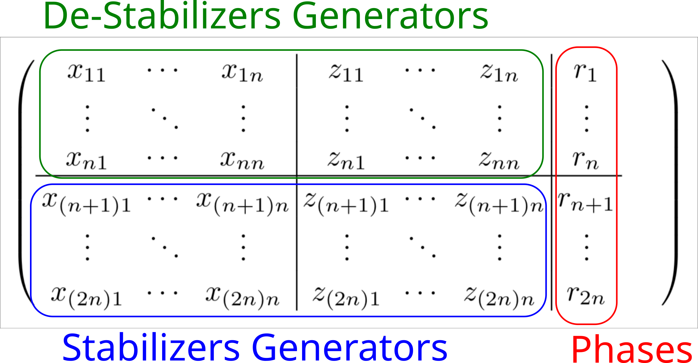
where \((x_{kl},z_{kl})\) are the bits encoding the \(n\)-qubits Pauli generator as
The qibo.quantum_info.clifford.Clifford object is in charge of storing the
phase-space representation of a stabilizer state.
This object is automatically created after the execution of a Clifford circuit through the
qibo.backends.clifford.CliffordBackend, but it can also be created by directly
passing a symplectic matrix to the constructor.
The generators of the stabilizers can be extracted with the
qibo.quantum_info.clifford.Clifford.generators() method,
or the complete set of \(d = 2^{n}\) stabilizers operators can be extracted through the
qibo.quantum_info.clifford.Clifford.stabilizers() method.
generators, phases = clifford.generators()
stabilizers = clifford.stabilizers()
The destabilizers can be extracted analogously with qibo.quantum_info.clifford.Clifford.destabilizers().
We provide integration with the stim package. It is possible to run Clifford circuits using stim as a platform:
from qibo.backends import CliffordBackend
from qibo.quantum_info import Clifford, random_clifford

clifford_backend = CliffordBackend(platform="stim")

circuit = random_clifford(nqubits)
result = clifford_backend.execute_circuit(circuit)

## Note that the execution above is equivalent to the one below

result = Clifford.from_circuit(circuit, platform="stim")
- class qibo.quantum_info.clifford.Clifford(data: _Buffer | _SupportsArray[dtype[Any]] | _NestedSequence[_SupportsArray[dtype[Any]]] | bool | int | float | complex | str | bytes | _NestedSequence[bool | int | float | complex | str | bytes] | Circuit, nqubits: int | None = None, measurements: list | None = None, nshots: int = 1000, platform: str | None = None, _backend: CliffordBackend | None = None, _measurement_gate: M = None, _samples: int | None = None)[source]#
Object storing the results of a circuit execution with the
qibo.backends.clifford.CliffordBackend.- Parameters:
data (ndarray or
qibo.models.circuit.Circuit) – Ifndarray, it is the symplectic matrix of the stabilizer state in phase-space representation. Ifqibo.models.circuit.Circuit, it is a circuit composed only of Clifford gates and computational-basis measurements.nqubits (int, optional) – number of qubits of the state.
measurements (list, optional) – list of measurements gates
qibo.gates.M. Defaults toNone.nshots (int, optional) – number of shots used for sampling the measurements. Defaults to \(1000\).
engine (str, optional) –
engine to use in the execution of the
qibo.backends.CliffordBackend. It accepts"numpy","numba","cupy", and"stim"(see stim). IfNone, defaults to the corresponding engine from the current backend. Defaults toNone.
- classmethod from_circuit(circuit: Circuit, initial_state: _Buffer | _SupportsArray[dtype[Any]] | _NestedSequence[_SupportsArray[dtype[Any]]] | bool | int | float | complex | str | bytes | _NestedSequence[bool | int | float | complex | str | bytes] | None = None, nshots: int = 1000, platform: str | None = None)[source]#
Allows to create a
qibo.quantum_info.clifford.Cliffordobject by executing the input circuit.- Parameters:
circuit (
qibo.models.circuit.Circuit) – Clifford circuit to run.initial_state (ndarray, optional) – symplectic matrix of the initial state. If
None, defaults to the symplectic matrix of the zero state. Defaults toNone.nshots (int, optional) – number of measurement shots to perform if
circuithas measurement gates. Defaults to \(10^{3}\).platform (str, optional) –
engine to use in the execution of the
qibo.backends.CliffordBackend. It accepts"numpy","numba","cupy", and"stim"(see stim). IfNone, defaults to the corresponding platform from the current backend. Defaults toNone.
- Returns:
Object storing the result of the circuit execution.
- Return type:
- to_circuit(algorithm: str | None = 'AG04', **kwargs) Circuit[source]#
Converts symplectic matrix into a Clifford circuit.
- Parameters:
algorithm (str, optional) – If
AG04, uses the decomposition algorithm from Aaronson & Gottesman (2004). IfBM20andClifford.nqubits <= 3, uses the decomposition algorithm from Bravyi & Maslov (2020). Defaults toAG04.kwargs (dict, optional) – Additional arguments used to initialize a Circuit object. For details, see the documentation of
qibo.models.circuit.Circuit.
- Returns:
circuit composed of Clifford gates.
- Return type:
- generators(return_array: bool = False) Tuple[List[str], List[int]] | Tuple[List[_Buffer | _SupportsArray[dtype[Any]] | _NestedSequence[_SupportsArray[dtype[Any]]] | bool | int | float | complex | str | bytes | _NestedSequence[bool | int | float | complex | str | bytes]], List[int]][source]#
Extracts the generators of stabilizers and destabilizers.
- stabilizers(symplectic: bool = False, return_array: bool = False) _Buffer | _SupportsArray[dtype[Any]] | _NestedSequence[_SupportsArray[dtype[Any]]] | bool | int | float | complex | str | bytes | _NestedSequence[bool | int | float | complex | str | bytes] | List[str][source]#
Extracts the stabilizers of the state.
- Parameters:
symplectic (bool, optional) – If
True, returns the rows of the symplectic matrix that correspond to the \(n\) generators of the \(2^{n}\) total stabilizers, independently ofreturn_array.return_array (bool, optional) – To be used when
symplectic = False. IfTruereturns the stabilizers asndarray. IfFalse, returns stabilizers as strings. Defaults toFalse.
- Returns:
Stabilizers of the state.
- Return type:
(ndarray or list)
- destabilizers(symplectic: bool = False, return_array: bool = False) _Buffer | _SupportsArray[dtype[Any]] | _NestedSequence[_SupportsArray[dtype[Any]]] | bool | int | float | complex | str | bytes | _NestedSequence[bool | int | float | complex | str | bytes] | List[str][source]#
Extracts the destabilizers of the state.
- Parameters:
symplectic (bool, optional) – If
True, returns the rows of the symplectic matrix that correspond to the \(n\) generators of the \(2^{n}\) total destabilizers, independently ofreturn_array.return_array (bool, optional) – To be used when
symplectic = False. IfTruereturns the destabilizers asndarray. IfFalse, their representation as strings is returned. Defaults toFalse.
- Returns:
Destabilizers of the state.
- Return type:
(ndarray or list)
- state() _Buffer | _SupportsArray[dtype[Any]] | _NestedSequence[_SupportsArray[dtype[Any]]] | bool | int | float | complex | str | bytes | _NestedSequence[bool | int | float | complex | str | bytes][source]#
Builds the density matrix representation of the state.
Note
This method is inefficient in runtime and memory for a large number of qubits.
- Returns:
Density matrix of the state.
- Return type:
(ndarray)
- property measurement_gate: M#
Single measurement gate containing all measured qubits.
Useful for sampling all measured qubits at once when simulating.
- samples(binary: bool = True, registers: bool = False) _Buffer | _SupportsArray[dtype[Any]] | _NestedSequence[_SupportsArray[dtype[Any]]] | bool | int | float | complex | str | bytes | _NestedSequence[bool | int | float | complex | str | bytes] | Dict[source]#
Returns raw measurement samples.
- Parameters:
- Returns:
- If
binaryisTrue samples are returned in binary form as a tensor of shape
(nshots, n_measured_qubits).- If
binaryisFalse samples are returned in decimal form as a tensor of shape
(nshots,).- If
registersisTrue samples are returned in a
dictwhere the keys are the register names and the values are the samples tensors for each register.- If
registersisFalse a single tensor is returned which contains samples from all the measured qubits, independently of their registers.
- If
- frequencies(binary: bool = True, registers: bool = False) _Buffer | _SupportsArray[dtype[Any]] | _NestedSequence[_SupportsArray[dtype[Any]]] | bool | int | float | complex | str | bytes | _NestedSequence[bool | int | float | complex | str | bytes] | Dict[source]#
Returns the frequencies of measured samples.
- Parameters:
- Returns:
A collections.Counter where the keys are the observed values and the values the corresponding frequencies, that is the number of times each measured value/bitstring appears.
- If
binaryisTrue the keys of the
collections.Counterare in binary form, as strings of \(0\) and :math`1`.- If
binaryisFalse the keys of the
collections.Counterare integers.- If
registersisTrue a dict of
collections.Counteris returned where keys are the name of each register.- If
registersisFalse a single
collections.Counteris returned which contains samples from all the measured qubits, independently of their registers.
- If
- probabilities(qubits: List[int] | Tuple[int, ...] | None = None) _Buffer | _SupportsArray[dtype[Any]] | _NestedSequence[_SupportsArray[dtype[Any]]] | bool | int | float | complex | str | bytes | _NestedSequence[bool | int | float | complex | str | bytes][source]#
Computes the probabilities of the selected qubits from the measured samples.
- copy(deep: bool = False)[source]#
Returns copy of
qibo.quantum_info.clifford.Cliffordobject.- Parameters:
deep (bool, optional) – If
True, creates another copy in memory. Defaults toFalse.- Returns:
copy of original
Cliffordobject.- Return type:
Entanglement measures#
Set of functions to calculate entanglement measures.
Concurrence#
- qibo.quantum_info.concurrence(state, bipartition, check_purity: bool = True, backend=None)[source]#
Calculates concurrence of a pure bipartite quantum state \(\rho \in \mathcal{H}_{A} \otimes \mathcal{H}_{B}\) as
\[C(\rho) = \sqrt{2 \, (\text{tr}^{2}(\rho) - \text{tr}(\rho_{A}^{2}))} \, ,\]where \(\rho_{A} = \text{tr}_{B}(\rho)\) is the reduced density operator obtained by tracing out the qubits in the
bipartition\(B\).- Parameters:
state (ndarray) – statevector or density matrix.
bipartition (list or tuple or ndarray) – qubits in the subsystem to be traced out.
check_purity (bool, optional) – if
True, checks ifstateis pure. IfFalse, it assumesstateis pure . Defaults toTrue.backend (
qibo.backends.abstract.Backend, optional) – backend to be used in the execution. IfNone, it uses the current backend. Defaults toNone.
- Returns:
Concurrence of \(\rho\).
- Return type:
Entanglement of formation#
- qibo.quantum_info.entanglement_of_formation(state, bipartition, base: float = 2, check_purity: bool = True, backend=None)[source]#
Calculates the entanglement of formation \(E_{f}\) of a pure bipartite quantum state \(\rho\), which is given by
\[E_{f} = H([1 - x, x]) \, ,\]where
\[x = \frac{1 + \sqrt{1 - C^{2}(\rho)}}{2} \, ,\]\(C(\rho)\) is the
qibo.quantum_info.concurrence()of \(\rho\), and \(H\) is theqibo.quantum_info.entropies.shannon_entropy().- Parameters:
state (ndarray) – statevector or density matrix.
bipartition (list or tuple or ndarray) – qubits in the subsystem to be traced out.
base (float) – the base of the log in
qibo.quantum_info.entropies.shannon_entropy(). Defaults to \(2\).check_purity (bool, optional) – if
True, checks ifstateis pure. IfFalse, it assumesstateis pure . Default:True.backend (
qibo.backends.abstract.Backend, optional) – backend to be used in the execution. IfNone, it uses the current backend. Defaults toNone.
- Returns:
entanglement of formation of state \(\rho\).
- Return type:
Negativity#
- qibo.quantum_info.negativity(state, bipartition, backend=None)[source]#
Calculates the negativity of a bipartite quantum state.
Given a bipartite state \(\rho \in \mathcal{H}_{A} \otimes \mathcal{H}_{B}\), the negativity \(\operatorname{Neg}(\rho)\) is given by
\[\operatorname{Neg}(\rho) = \frac{1}{2} \, \left( \norm{\rho_{B}}_{1} - 1 \right) \, ,\]where \(\rho_{B}\) is the reduced density matrix after tracing out qubits in partition \(A\), and \(\norm{\cdot}_{1}\) is the Schatten \(1\)-norm (also known as nuclear norm or trace norm).
- Parameters:
state (ndarray) – statevector or density matrix.
bipartition (list or tuple or ndarray) – qubits in the subsystem to be traced out.
backend (
qibo.backends.abstract.Backend, optional) – backend to be used in the execution. IfNone, it uses it uses the current backend. Defaults toNone.
- Returns:
Negativity \(\operatorname{Neg}(\rho)\) of state \(\rho\).
- Return type:
Entanglement fidelity#
- qibo.quantum_info.entanglement_fidelity(channel, nqubits: int, state=None, backend=None)[source]#
Entanglement fidelity \(F_{\mathcal{E}}\) of a
channel\(\mathcal{E}\) onstate\(\rho\) is given by\[F_{\mathcal{E}}(\rho) = F(\rho_{f}, \rho)\]where \(F\) is the
qibo.quantum_info.fidelity()function for states, and \(\rho_{f} = \mathcal{E}_{A} \otimes I_{B}(\rho)\) is the state after the channel \(\mathcal{E}\) was applied to partition \(A\).- Parameters:
channel (
qibo.gates.channels.Channel) – quantum channel acting on partition \(A\).nqubits (int) – total number of qubits in
state.state (ndarray, optional) – statevector or density matrix to be evolved by
channel. IfNone, defaults to the maximally entangled state \(\frac{1}{2^{n}} \, \sum_{k} \, \ket{k}\ket{k}\), where \(n\) isnqubits. Defaults toNone.backend (
qibo.backends.abstract.Backend, optional) – backend to be used in the execution. IfNone, it uses the current backend. Defaults toNone.
- Returns:
Entanglement fidelity \(F_{\mathcal{E}}\).
- Return type:
Meyer-Wallach entanglement#
- qibo.quantum_info.meyer_wallach_entanglement(state, backend=None)[source]#
Compute the Meyer-Wallach entanglement \(Q\) of a
state,\[Q(\rho) = 2\left(1 - \frac{1}{N} \, \sum_{k} \, \text{tr}\left(\rho_{k}^{2}\right)\right) \, ,\]where \(\rho_{k}^{2}\) is the reduced density matrix of qubit \(k\), and \(N\) is the total number of qubits in
state. We use the definition of the Meyer-Wallach entanglement as the average purity proposed in Brennen (2003), which is equivalent to the definition introduced in Meyer and Wallach (2002).- Parameters:
state (ndarray) – statevector or density matrix.
backend (
qibo.backends.abstract.Backend, optional) – backend to be used in the execution. IfNone, it uses the current backend. Defaults toNone.
- Returns:
Meyer-Wallach entanglement \(Q\).
- Return type:
References
1. G. K. Brennen, An observable measure of entanglement for pure states of multi-qubit systems, Quantum Information and Computation, vol. 3 (6), 619-626 (2003).
2. D. A. Meyer and N. R. Wallach, Global entanglement in multiparticle systems, J. Math. Phys. 43, 4273–4278 (2002).
Entanglement capability#
- qibo.quantum_info.entangling_capability(circuit, samples: int, seed: int | None = None, backend: Backend | None = None)[source]#
Return the entangling capability \(\text{Ent}\) of a parametrized circuit.
It is defined as the average Meyer-Wallach entanglement \(Q\) (
qibo.quantum_info.meyer_wallach_entanglement()) of thecircuit, i.e.\[\text{Ent} = \frac{2}{|\mathcal{S}|}\sum_{\theta_{k} \in \mathcal{S}} \, Q(\rho_{k}) \, ,\]where \(\mathcal{S}\) is the set of sampled circuit parameters, and \(\rho_{k}\) is the state prepared by the circuit with uniformily-sampled parameters \(\theta_{k}\).
Note
Currently, function does not work with
circuitthat contains noisy channels.- Parameters:
circuit (
qibo.models.Circuit) – Parametrized circuit.samples (int) – number of sampled circuit parameter vectors \(|S|\)
seed (int or
numpy.random.Generator, optional) – Either a generator of random numbers or a fixed seed to initialize a generator. IfNone, initializes a generator with a random seed. Default:None.backend (
qibo.backends.abstract.Backend, optional) – backend to be used in the execution. IfNone, it uses the current backend. Defaults toNone.
- Returns:
Entangling capability \(\text{Ent}\).
- Return type:
Entropy measures#
Set of functions to calculate entropy measures.
Shannon entropy#
- qibo.quantum_info.shannon_entropy(prob_dist, base: float = 2, backend=None)[source]#
Calculate the Shannon entropy of a probability array \(\mathbf{p}\), which is given by
\[H(\mathbf{p}) = - \sum_{k = 0}^{d^{2} - 1} \, p_{k} \, \log_{b}(p_{k}) \, ,\]where \(d = \text{dim}(\mathcal{H})\) is the dimension of the Hilbert space \(\mathcal{H}\), \(b\) is the log base (default 2), and \(0 \log_{b}(0) \equiv 0\).
- Parameters:
prob_dist (ndarray or list) – a probability array \(\mathbf{p}\).
base (float) – the base of the log. Defaults to \(2\).
backend (
qibo.backends.abstract.Backend, optional) – backend to be used in the execution. IfNone, it uses the current backend. Defaults toNone.
- Returns:
Shannon entropy \(H(\mathcal{p})\).
- Return type:
Classical relative entropy#
- qibo.quantum_info.classical_relative_entropy(prob_dist_p, prob_dist_q, base: float = 2, backend=None)[source]#
Calculates the relative entropy between two discrete probability distributions.
For probabilities \(\mathbf{p}\) and \(\mathbf{q}\), it is defined as
\[D(\mathbf{p} \, \| \, \mathbf{q}) = \sum_{x} \, \mathbf{p}(x) \, \log\left( \frac{\mathbf{p}(x)}{\mathbf{q}(x)} \right) \, .\]The classical relative entropy is also known as the Kullback-Leibler (KL) divergence.
- Parameters:
prob_dist_p (ndarray or list) – discrete probability distribution \(p\).
prob_dist_q (ndarray or list) – discrete probability distribution \(q\).
base (float) – the base of the log. Defaults to \(2\).
backend (
qibo.backends.abstract.Backend, optional) – backend to be used in the execution. IfNone, it uses the current backend. Defaults toNone.
- Returns:
Classical relative entropy between \(\mathbf{p}\) and \(\mathbf{q}\).
- Return type:
Classical mutual information#
- qibo.quantum_info.classical_mutual_information(prob_dist_joint, prob_dist_p, prob_dist_q, base: float = 2, backend=None)[source]#
Calculates the classical mutual information of two random variables.
Given two random variables \((X, \, Y)\), their mutual information is given by
\[I(X, \, Y) \equiv H(p(x)) + H(q(y)) - H(p(x, \, y)) \, ,\]where \(p(x, \, y)\) is the joint probability distribution of \((X, Y)\), \(p(x)\) is the marginal probability distribution of \(X\), \(q(y)\) is the marginal probability distribution of \(Y\), and \(H(\cdot)\) is the
qibo.quantum_info.entropies.shannon_entropy().- Parameters:
prob_dist_joint (ndarray) – joint probability distribution \(p(x, \, y)\).
prob_dist_p (ndarray) – marginal probability distribution \(p(x)\).
prob_dist_q (ndarray) – marginal probability distribution \(q(y)\).
base (float) – the base of the log. Defaults to \(2\).
backend (
qibo.backends.abstract.Backend, optional) – backend to be used in the execution. IfNone, it uses the current backend. Defaults toNone.
- Returns:
Mutual information \(I(X, \, Y)\).
- Return type:
Classical Rényi entropy#
- qibo.quantum_info.classical_renyi_entropy(prob_dist, alpha: float | int, base: float = 2, backend=None)[source]#
Calculates the classical Rényi entropy \(H_{\alpha}\) of a discrete probability distribution.
For \(\alpha \in (0, \, 1) \cup (1, \, \infty)\) and probability distribution \(\mathbf{p}\), the classical Rényi entropy is defined as
\[H_{\alpha}(\mathbf{p}) = \frac{1}{1 - \alpha} \, \log\left( \sum_{x} \, \mathbf{p}^{\alpha}(x) \right) \, .\]A special case is the limit \(\alpha \to 1\), in which the classical Rényi entropy coincides with the
qibo.quantum_info.entropies.shannon_entropy().Another special case is the limit \(\alpha \to 0\), where the function is reduced to \(\log\left(|\mathbf{p}|\right)\), with \(|\mathbf{p}|\) being the support of \(\mathbf{p}\). This is known as the Hartley entropy (also known as Hartley function or max-entropy).
In the limit \(\alpha \to \infty\), the function reduces to \(-\log(\max_{x}(\mathbf{p}(x)))\), which is called the min-entropy.
- Parameters:
prob_dist (ndarray) – discrete probability distribution.
base (float) – the base of the log. Defaults to \(2\).
backend (
qibo.backends.abstract.Backend, optional) – backend to be used in the execution. IfNone, it uses the current backend. Defaults toNone.
- Returns:
Classical Rényi entropy \(H_{\alpha}\).
- Return type:
Classical Rényi relative entropy#
- qibo.quantum_info.classical_relative_renyi_entropy(prob_dist_p, prob_dist_q, alpha: float | int, base: float = 2, backend=None)[source]#
Calculates the classical relative Rényi entropy between two discrete probability distributions.
This function is also known as Rényi divergence.
For \(\alpha \in (0, \, 1) \cup (1, \, \infty)\) and probability distributions \(\mathbf{p}\) and \(\mathbf{q}\), the classical relative Rényi entropy is defined as
\[H_{\alpha}(\mathbf{p} \, \| \, \mathbf{q}) = \frac{1}{\alpha - 1} \, \log\left( \sum_{x} \, \frac{\mathbf{p}^{\alpha}(x)} {\mathbf{q}^{\alpha - 1}(x)} \right) \, .\]A special case is the limit \(\alpha \to 1\), in which the classical Rényi divergence coincides with the
qibo.quantum_info.entropies.classical_relative_entropy().Another special case is the limit \(\alpha \to 1/2\), where the function is reduced to \(-2 \log\left(\sum_{x} \, \sqrt{\mathbf{p}(x) \, \mathbf{q}(x)} \right)\). The sum inside the \(\log\) is known as the Bhattacharyya coefficient.
In the limit \(\alpha \to \infty\), the function reduces to \(\log(\max_{x}(\mathbf{p}(x) \, \mathbf{q}(x))\).
- Parameters:
prob_dist_p (ndarray or list) – discrete probability distribution \(p\).
prob_dist_q (ndarray or list) – discrete probability distribution \(q\).
base (float) – the base of the log. Defaults to \(2\).
backend (
qibo.backends.abstract.Backend, optional) – backend to be used in the execution. IfNone, it uses the current backend. Defaults toNone.
- Returns:
Classical relative Rényi entropy \(H_{\alpha}(\mathbf{p} \, \| \, \mathbf{q})\).
- Return type:
Classical Tsallis entropy#
- qibo.quantum_info.classical_tsallis_entropy(prob_dist, alpha: float, base: float = 2, backend=None)[source]#
Calculates the classical Tsallis entropy for a discrete probability distribution.
This is defined as
\[S_{\alpha}(\mathbf{p}) = \frac{1}{\alpha - 1} \, \left(1 - \sum_{x} \, \mathbf{p}^{\alpha}(x) \right)\]- Parameters:
prob_dist (ndarray) – discrete probability distribution.
base (float) – the base of the log. Used when
alpha=1.0. Defaults to \(2\).backend (
qibo.backends.abstract.Backend, optional) – backend to be used in the execution. IfNone, it uses the current backend. Defaults toNone.
- Returns:
Classical Tsallis entropy \(S_{\alpha}(\mathbf{p})\).
- Return type:
Classical Tsallis relative entropy#
- qibo.quantum_info.classical_relative_tsallis_entropy(prob_dist_p, prob_dist_q, alpha: float, base: float = 2, backend=None)[source]#
Calculate the classical relative Tsallis entropy between two discrete probability distributions.
Given a discrete random variable \(\chi\) that has values \(x\) in the set \(\mathcal{X}\) with probability \(\mathrm{p}(x)\) and a discrete random variable \(\upsilon\) that has the values \(x\) in the same set \(\mathcal{X}\) with probability \(\mathrm{q}(x)\), their relative Tsallis entropy is given by
\[D_{\alpha}^{\text{ts}}(\chi \, \| \, \upsilon) = \sum_{x \in \mathcal{X}} \, \mathrm{p}^{\alpha}(x) \, \ln_{\alpha} \left( \frac{\mathrm{p}(x)}{\mathrm{q}(x)} \right) \, ,\]where \(\ln_{\alpha}(x) \equiv \frac{x^{1 - \alpha} - 1}{1 - \alpha}\) is the so-called \(\alpha\)-logarithm. When \(\alpha = 1\), it reduces to
qibo.quantum_info.entropies.classical_relative_entropy.- Parameters:
prob_dist_p (ndarray or list) – discrete probability distribution \(p\).
prob_dist_q (ndarray or list) – discrete probability distribution \(q\).
alpha (float) – entropic index.
base (float) – the base of the log used when \(\alpha = 1\). Defaults to \(2\).
backend (
qibo.backends.abstract.Backend, optional) – backend to be used in the execution. IfNone, it uses the current backend. Defaults toNone.
- Returns:
Tsallis relative entropy \(D_{\alpha}^{\text{ts}}\).
- Return type:
von Neumann entropy#
- qibo.quantum_info.von_neumann_entropy(state, base: float = 2, return_spectrum: bool = False, backend=None)[source]#
Calculate the von-Neumann entropy \(S(\rho)\) of a quantum
state\(\rho\).It is given by
\[S(\rho) = - \text{tr}\left(\rho \, \log(\rho)\right)\]- Parameters:
state (ndarray) – statevector or density matrix.
base (float, optional) – the base of the log. Defaults to \(2\).
return_spectrum – if
True, returnsentropyand \(-\log_{\textup{b}}(\textup{eigenvalues})\), where \(b\) isbase. IfFalse, returns onlyentropy. Default isFalse.backend (
qibo.backends.abstract.Backend, optional) – backend to be used in the execution. IfNone, it uses the current backend. Defaults toNone.
- Returns:
The von-Neumann entropy \(S\) of
state\(\rho\).- Return type:
Relative von Neumann entropy#
- qibo.quantum_info.relative_von_neumann_entropy(state, target, base: float = 2, backend=None)[source]#
Calculates the relative von Neumann entropy between two quantum states.
Also known as quantum relative entropy, \(S(\rho \, \| \, \sigma)\) is given by
\[S(\rho \, \| \, \sigma) = \text{tr}\left(\rho \, \log(\rho)\right) - \text{tr}\left(\rho \, \log(\sigma)\right)\]where
state\(\rho\) andtarget\(\sigma\) are two quantum states.- Parameters:
state (ndarray) – statevector or density matrix \(\rho\).
target (ndarray) – statevector or density matrix \(\sigma\).
base (float, optional) – the base of the log. Defaults to \(2\).
backend (
qibo.backends.abstract.Backend, optional) – backend to be used in the execution. IfNone, it uses the current backend. Defaults toNone.
- Returns:
Relative von-Neumann entropy \(S(\rho \, \| \, \sigma)\).
- Return type:
Mutual information#
- qibo.quantum_info.mutual_information(state, partition, base: float = 2, backend=None)[source]#
Calculates the mutual information of a bipartite state.
Given a qubit
partition\(A\), the mutual information of state \(\rho\) is given by\[I(\rho) \equiv S(\rho_{A}) + S(\rho_{B}) - S(\rho) \, ,\]where \(B\) is the remaining qubits that are not in partition \(A\), and \(S(\cdot)\) is the
qibo.quantum_info.von_neumann_entropy().- Parameters:
state (ndarray) – statevector or density matrix.
partition (Union[List[int], Tuple[int]]) – indices of qubits in partition \(A\).
base (float, optional) – the base of the log. Defaults to \(2\).
backend (
qibo.backends.abstract.Backend, optional) – backend to be used in the execution. IfNone, it uses the current backend. Defaults toNone.
- Returns:
Mutual information \(I(\rho)\) of
state\(\rho\).- Return type:
Rényi entropy#
- qibo.quantum_info.renyi_entropy(state, alpha: float | int, base: float = 2, backend=None)[source]#
Calculates the Rényi entropy \(H_{\alpha}\) of a quantum state \(\rho\).
For \(\alpha \in (0, \, 1) \cup (1, \, \infty)\), the Rényi entropy is defined as
\[H_{\alpha}(\rho) = \frac{1}{1 - \alpha} \, \log\left( \rho^{\alpha} \right) \, .\]A special case is the limit \(\alpha \to 1\), in which the Rényi entropy coincides with the
qibo.quantum_info.entropies.entropy().Another special case is the limit \(\alpha \to 0\), where the function is reduced to \(\log\left(d\right)\), with \(d = 2^{n}\) being the dimension of the Hilbert space in which
state\(\rho\) lives in. This is known as the Hartley entropy (also known as Hartley function or max-entropy).In the limit \(\alpha \to \infty\), the function reduces to \(-\log(\|\rho\|_{\infty})\), with \(\|\cdot\|_{\infty}\) being the spectral norm. This is known as the min-entropy.
- Parameters:
state (ndarray) – statevector or density matrix.
base (float) – the base of the log. Defaults to \(2\).
backend (
qibo.backends.abstract.Backend, optional) – backend to be used in the execution. IfNone, it uses the current backend. Defaults toNone.
- Returns:
Rényi entropy \(H_{\alpha}\).
- Return type:
Relative Rényi entropy#
- qibo.quantum_info.relative_renyi_entropy(state, target, alpha: float | int, base: float = 2, backend=None)[source]#
Calculates the relative Rényi entropy between two quantum states.
For \(\alpha \in (0, \, 1) \cup (1, \, \infty)\) and quantum states \(\rho\) and \(\sigma\), the relative Rényi entropy is defined as
\[H_{\alpha}(\rho \, \| \, \sigma) = \frac{1}{\alpha - 1} \, \log\left( \textup{tr}\left( \rho^{\alpha} \, \sigma^{1 - \alpha} \right) \right) \, .\]A special case is the limit \(\alpha \to 1\), in which the Rényi entropy coincides with the
qibo.quantum_info.entropies.relative_von_neumann_entropy().In the limit \(\alpha \to \infty\), the function reduces to \(-2 \, \log(\|\sqrt{\rho} \, \sqrt{\sigma}\|_{1})\), with \(\|\cdot\|_{1}\) being the Schatten 1-norm. This is known as the min-relative entropy.
Note
Function raises
NotImplementedErrorwhentarget\(\sigma\) is a pure state and \(\alpha > 1\). This is due to the fact that it is not possible to calculate \(\sigma^{1 - \alpha}\) when \(\alpha > 1\) and \(\sigma\) is a projector, i.e. a singular matrix.- Parameters:
state (ndarray) – statevector or density matrix \(\rho\).
target (ndarray) – statevector or density matrix \(\sigma\).
base (float) – the base of the log. Defaults to \(2\).
backend (
qibo.backends.abstract.Backend, optional) – backend to be used in the execution. IfNone, it uses the current backend. Defaults toNone.
- Returns:
Relative Rényi entropy \(H_{\alpha}(\rho \, \| \, \sigma)\).
- Return type:
Tsallis entropy#
- qibo.quantum_info.tsallis_entropy(state, alpha: float, base: float = 2, backend=None)[source]#
Calculates the Tsallis entropy of a quantum state.
\[S_{\alpha}(\rho) = \frac{1}{1 - \alpha} \, \left( \text{tr}(\rho^{\alpha}) - 1 \right)\]When \(\alpha = 1\), the functions defaults to
qibo.quantum_info.entropies.entropy().- Parameters:
state (ndarray) – statevector or density matrix.
base (float, optional) – the base of the log. Used when
alpha=1.0. Defaults to \(2\).backend (
qibo.backends.abstract.Backend, optional) – backend to be used in the execution. IfNone, it uses the current backend. Defaults toNone.
- Returns:
Tsallis entropy \(S_{\alpha}(\rho)\).
- Return type:
Relative Tsallis entropy#
- qibo.quantum_info.relative_tsallis_entropy(state, target, alpha: float | int, base: float = 2, backend=None)[source]#
Calculate the relative Tsallis entropy between two quantum states.
For \(\alpha \in [0, \, 2]\) and quantum states \(\rho\) and \(\sigma\), the relative Tsallis entropy is defined as
\[\Delta_{\alpha}^{\text{ts}}(\rho, \, \sigma) = \frac{1 - \text{tr}\left(\rho^{\alpha} \, \sigma^{1 - \alpha}\right)}{1 - \alpha} \, .\]A special case is the limit \(\alpha \to 1\), in which the Tsallis entropy coincides with the
qibo.quantum_info.entropies.relative_von_neumann_entropy().- Parameters:
state (ndarray) – statevector or density matrix \(\rho\).
target (ndarray) – statevector or density matrix \(\sigma\).
alpha (float or int) – entropic index \(\alpha \in [0, \, 2]\).
base (float, optional) – the base of the log used when \(\alpha = 1\). Defaults to \(2\).
backend (
qibo.backends.abstract.Backend, optional) – backend to be used in the execution. IfNone, it usesqibo.backends.GlobalBackend. Defaults toNone.
- Returns:
Relative Tsallis entropy \(\Delta_{\alpha}^{\text{ts}}\).
- Return type:
References
1. S. Abe, Nonadditive generalization of the quantum Kullback-Leibler divergence for measuring the degree of purification, Phys. Rev. A 68, 032302.
2. S. Furuichi, K. Yanagi, and K. Kuriyama, Fundamental properties of Tsallis relative entropy, J. Math. Phys., Vol. 45, Issue 12, pp. 4868-4877 (2004) .
Entanglement entropy#
- qibo.quantum_info.entanglement_entropy(state, bipartition, base: float = 2, return_spectrum: bool = False, backend=None)[source]#
Calculates the entanglement entropy \(S\) of bipartition \(A\) of
state\(\rho\). This is given by\[S(\rho_{A}) = -\text{tr}(\rho_{A} \, \log(\rho_{A})) \, ,\]where \(\rho_{A} = \text{tr}_{B}(\rho)\) is the reduced density matrix calculated by tracing out the
bipartition\(B\).- Parameters:
state (ndarray) – statevector or density matrix.
bipartition (list or tuple or ndarray) – qubits in the subsystem to be traced out.
base (float, optional) – the base of the log. Defaults to :math: 2.
return_spectrum – if
True, returnsentropyand eigenvalues ofstate. IfFalse, returns onlyentropy. Default isFalse.backend (
qibo.backends.abstract.Backend, optional) – backend to be used in the execution. IfNone, it uses the current backend. Defaults toNone.
- Returns:
Entanglement entropy \(S\) of
state\(\rho\).- Return type:
Metrics#
Set of functions that are used to calculate metrics of states, (pseudo-)distance measures between states, and distance measures between quantum channels.
Purity#
- qibo.quantum_info.purity(state: _Buffer | _SupportsArray[dtype[Any]] | _NestedSequence[_SupportsArray[dtype[Any]]] | bool | int | float | complex | str | bytes | _NestedSequence[bool | int | float | complex | str | bytes], backend: Backend | None = None) float[source]#
Purity of a quantum state \(\rho\).
This is given by
\[\text{purity}(\rho) = \text{tr}(\rho^{2}) \, .\]- Parameters:
state (ArrayLike) – statevector or density matrix.
backend (
qibo.backends.abstract.Backend, optional) – backend to be used in the execution. IfNone, it uses the current backend. Defaults toNone.
- Returns:
Purity of quantum
state\(\rho\).- Return type:
Impurity#
- qibo.quantum_info.impurity(state: _Buffer | _SupportsArray[dtype[Any]] | _NestedSequence[_SupportsArray[dtype[Any]]] | bool | int | float | complex | str | bytes | _NestedSequence[bool | int | float | complex | str | bytes], backend: Backend | None = None) float[source]#
Impurity of quantum state \(\rho\).
This is given by \(1 - \text{purity}(\rho)\), where \(\text{purity}\) is defined in
qibo.quantum_info.purity().- Parameters:
state (ArrayLike) – statevector or density matrix.
backend (
qibo.backends.abstract.Backend, optional) – backend to be used in the execution. IfNone, it uses the current backend. Defaults toNone.
- Returns:
Impurity of
state\(\rho\).- Return type:
Trace distance#
- qibo.quantum_info.trace_distance(state: _Buffer | _SupportsArray[dtype[Any]] | _NestedSequence[_SupportsArray[dtype[Any]]] | bool | int | float | complex | str | bytes | _NestedSequence[bool | int | float | complex | str | bytes], target: _Buffer | _SupportsArray[dtype[Any]] | _NestedSequence[_SupportsArray[dtype[Any]]] | bool | int | float | complex | str | bytes | _NestedSequence[bool | int | float | complex | str | bytes], backend: Backend | None = None) float[source]#
Trace distance between two quantum states, \(\rho\) and \(\sigma\):
\[T(\rho, \sigma) = \frac{1}{2} \, \|\rho - \sigma\|_{1} = \frac{1}{2} \, \text{tr}\left[ \sqrt{(\rho - \sigma)^{\dagger}(\rho - \sigma)} \right] \, ,\]where \(\|\cdot\|_{1}\) is the Schatten 1-norm.
- Parameters:
state (ArrayLike) – statevector or density matrix.
target (ArrayLike) – statevector or density matrix.
backend (
qibo.backends.abstract.Backend, optional) – backend to be used in the execution. IfNone, it uses the current backend. Defaults toNone.
- Returns:
Trace distance between
state\(\rho\) andtarget\(\sigma\).- Return type:
Hilbert-Schmidt inner product#
- qibo.quantum_info.hilbert_schmidt_inner_product(operator_A: _Buffer | _SupportsArray[dtype[Any]] | _NestedSequence[_SupportsArray[dtype[Any]]] | bool | int | float | complex | str | bytes | _NestedSequence[bool | int | float | complex | str | bytes], operator_B: _Buffer | _SupportsArray[dtype[Any]] | _NestedSequence[_SupportsArray[dtype[Any]]] | bool | int | float | complex | str | bytes | _NestedSequence[bool | int | float | complex | str | bytes], backend: Backend | None = None) float[source]#
Calculate the Hilbert-Schmidt inner product between two operators.
Given two operators \(A, \, B \in \mathcal{H}\), the Hilbert-Schmidt inner product between the two is given by
\[\braket{A, \, B}_{\text{HS}} = \text{tr}\left(A^{\dagger} \, B\right) \, .\]- Parameters:
operator_A (ArrayLike) – operator \(A\).
operator_B (ArrayLike) – operator \(B\).
backend (
qibo.backends.abstract.Backend, optional) – backend to be used in the execution. IfNone, it uses the current backend. Defaults toNone.
- Returns:
Hilbert-Schmidt inner product \(\braket{A, \, B}_{\text{HS}}\).
- Return type:
Hilbert-Schmidt distance#
- qibo.quantum_info.hilbert_schmidt_distance(state: _Buffer | _SupportsArray[dtype[Any]] | _NestedSequence[_SupportsArray[dtype[Any]]] | bool | int | float | complex | str | bytes | _NestedSequence[bool | int | float | complex | str | bytes], target: _Buffer | _SupportsArray[dtype[Any]] | _NestedSequence[_SupportsArray[dtype[Any]]] | bool | int | float | complex | str | bytes | _NestedSequence[bool | int | float | complex | str | bytes], backend: Backend | None = None) float[source]#
Calculate the Hilbert-Schmidt distance between two quantum states:
\[\braket{\rho - \sigma, \, \rho - \sigma}_{\text{HS}} = \text{tr}\left((\rho - \sigma)^{2}\right) \, ,\]where \(\braket{\cdot, \, \cdot}_{\text{HS}}\) is the
qibo.quantum_info.hilbert_schmidt_inner_product().- Parameters:
state (ArrayLike) – statevector or density matrix.
target (ArrayLike) – statevector or density matrix.
backend (
qibo.backends.abstract.Backend, optional) – backend to be used in the execution. IfNone, it uses the current backend. Defaults toNone.
- Returns:
Hilbert-Schmidt distance between
state\(\rho\) andtarget\(\sigma\).- Return type:
References
1. P. J. Coles, M. Cerezo, and L. Cincio, Strong bound between trace distance and Hilbert-Schmidt distance for low-rank states, Phys. Rev. A 100, 022103 (2019).
Fidelity#
- qibo.quantum_info.fidelity(state: _Buffer | _SupportsArray[dtype[Any]] | _NestedSequence[_SupportsArray[dtype[Any]]] | bool | int | float | complex | str | bytes | _NestedSequence[bool | int | float | complex | str | bytes], target: _Buffer | _SupportsArray[dtype[Any]] | _NestedSequence[_SupportsArray[dtype[Any]]] | bool | int | float | complex | str | bytes | _NestedSequence[bool | int | float | complex | str | bytes], precision_tol: float = 1e-08, backend: Backend | None = None) float[source]#
Fidelity \(F(\rho, \sigma)\) between
state\(\rho\) andtargetstate \(\sigma\). In general,\[F(\rho, \sigma) = \text{tr}^{2}\left( \sqrt{\sqrt{\sigma} \, \rho^{\dagger} \, \sqrt{\sigma}} \right) \, .\]However, when at least one of the states is pure, then
\[F(\rho, \sigma) = \text{tr}(\rho \, \sigma)\]- Parameters:
state (ndarray) – statevector or density matrix.
target (ndarray) – statevector or density matrix.
precision_tol (float, optional) – precision tolerance in
qibo.quantum_info.impurity()used to decide ifstateandtargetare pure or mixed states. Defaults to \(10^{-8}\).backend (
qibo.backends.abstract.Backend, optional) – backend to be used in the execution. IfNone, it uses the current backend. Defaults toNone.
- Returns:
Fidelity between
state\(\rho\) andtarget\(\sigma\).- Return type:
Infidelity#
- qibo.quantum_info.infidelity(state: _Buffer | _SupportsArray[dtype[Any]] | _NestedSequence[_SupportsArray[dtype[Any]]] | bool | int | float | complex | str | bytes | _NestedSequence[bool | int | float | complex | str | bytes], target: _Buffer | _SupportsArray[dtype[Any]] | _NestedSequence[_SupportsArray[dtype[Any]]] | bool | int | float | complex | str | bytes | _NestedSequence[bool | int | float | complex | str | bytes], backend: Backend | None = None) float[source]#
Infidelity between
state\(\rho\) andtargetstate \(\sigma\), which is given by\[1 - F(\rho, \, \sigma) \, ,\]where \(F(\rho, \, \sigma)\) is the
qibo.quantum_info.fidelity()betweenstateandtarget.- Parameters:
state (ArrayLike) – statevector or density matrix.
target (ArrayLike) – statevector or density matrix.
backend (
qibo.backends.abstract.Backend, optional) – backend to be used in the execution. IfNone, it uses the current backend. Defaults toNone.
- Returns:
Infidelity between
state\(\rho\) andtarget\(\sigma\).- Return type:
A fidelity#
- qibo.quantum_info.a_fidelity(state: _Buffer | _SupportsArray[dtype[Any]] | _NestedSequence[_SupportsArray[dtype[Any]]] | bool | int | float | complex | str | bytes | _NestedSequence[bool | int | float | complex | str | bytes], target: _Buffer | _SupportsArray[dtype[Any]] | _NestedSequence[_SupportsArray[dtype[Any]]] | bool | int | float | complex | str | bytes | _NestedSequence[bool | int | float | complex | str | bytes], backend: Backend | None = None) float[source]#
Return the \(A\)-fidelity between two quantum states.
For a quantum
state\(\rho\) and atargetquantum state \(\sigma\), the \(A\)-fidelity is defined as:\[F_{\text{A}}(\rho, \, \sigma) = \text{tr}^{2}(\sqrt{\rho} \, \sqrt{\sigma}) \, .\]- Parameters:
state (ArrayLike) – statevector or density matrix.
target (ArrayLike) – statevector or density matrix.
backend (
qibo.backends.abstract.Backend, optional) – backend to be used in the execution. IfNone, it uses the current backend. Defaults toNone.
- Returns:
\(A\)-fidelity between \(\rho\) and \(\sigma\).
- Return type:
References
1. Y.-C. Liang, Y.-H. Yeh, P. E. M. F. Mendonça, R. Y. Teh, M. D. Reid, and P. D. Drummond, Quantum fidelity measures for mixed states, Rep. Prog. Phys. 82 076001 (2019).
2. Z. Ma, F.-L. Zhang, and J.-L. Chen. Geometric interpretation for the A fidelity and its relation with the Bures fidelity, Phys. Rev. A, 78(6):064305, (2008).
N fidelity#
- qibo.quantum_info.n_fidelity(state: _Buffer | _SupportsArray[dtype[Any]] | _NestedSequence[_SupportsArray[dtype[Any]]] | bool | int | float | complex | str | bytes | _NestedSequence[bool | int | float | complex | str | bytes], target: _Buffer | _SupportsArray[dtype[Any]] | _NestedSequence[_SupportsArray[dtype[Any]]] | bool | int | float | complex | str | bytes | _NestedSequence[bool | int | float | complex | str | bytes], backend: Backend | None = None) float[source]#
Return the \(N\)-fidelity between two quantum states.
For a quantum
state\(\rho\) and atargetquantum state \(\sigma\), the \(N\)-fidelity is defined as:\[F_{\text{N}}(\rho, \, \sigma) = \text{tr}(\rho \, \sigma) + \sqrt{1 - \text{tr}(\rho^{2})} \, \sqrt{1 - \text{tr}(\rho^{2})} \, ,\]where \(\text{tr}(\varrho^{2})\) is the
qibo.quantum_info.purityof a quantum state \(\varrho\).- Parameters:
state (ArrayLike) – statevector or density matrix.
target (ArrayLike) – statevector or density matrix.
backend (
qibo.backends.abstract.Backend, optional) – backend to be used in the execution. IfNone, it uses the current backend. Defaults toNone.
- Returns:
\(N\)-fidelity between \(\rho\) and \(\sigma\).
- Return type:
References
1. Y.-C. Liang, Y.-H. Yeh, P. E. M. F. Mendonça, R. Y. Teh, M. D. Reid, and P. D. Drummond, Quantum fidelity measures for mixed states, Rep. Prog. Phys. 82 076001 (2019).
2. P. E. M. F. Mendonça, R. d. J. Napolitano, M. A. Marchiolli, C. J. Foster, and Y.-C. Liang. Alternative fidelity measure between quantum states, Phys. Rev. A, 78 052330 (2008).
3. A. Miszczak, Z. Puchala, P. Horodecki, A. Uhlmann, and K. Zyczkowski. Sub- and super-fidelity as bounds for quantum fidelity. Quantum Inf. Comput., 9(1):103–130, (2009).
Chen fidelity#
- qibo.quantum_info.chen_fidelity(state: _Buffer | _SupportsArray[dtype[Any]] | _NestedSequence[_SupportsArray[dtype[Any]]] | bool | int | float | complex | str | bytes | _NestedSequence[bool | int | float | complex | str | bytes], target: _Buffer | _SupportsArray[dtype[Any]] | _NestedSequence[_SupportsArray[dtype[Any]]] | bool | int | float | complex | str | bytes | _NestedSequence[bool | int | float | complex | str | bytes], backend: Backend | None = None) float[source]#
Return the Chen fidelity between two quantum states.
For a quantum
state\(\rho\) and atargetquantum state \(\sigma\), the Chen fidelity is defined as:\[F_{\text{C}}(\rho, \, \sigma) = \frac{1 - r}{2} + \frac{1 + r}{2} \, F_{\text{N}}(\rho, \, \sigma) \, ,\]where \(\text{tr}(\varrho^{2})\) is the
qibo.quantum_info.purityof a quantum state \(\varrho\).- Parameters:
state (ndarray) – statevector or density matrix.
target (ndarray) – statevector or density matrix.
backend (
qibo.backends.abstract.Backend, optional) – backend to be used in the execution. IfNone, it uses the current backend. Defaults toNone.
- Returns:
Chen fidelity between \(\rho\) and \(\sigma\).
- Return type:
References
1. Y.-C. Liang, Y.-H. Yeh, P. E. M. F. Mendonça, R. Y. Teh, M. D. Reid, and P. D. Drummond, Quantum fidelity measures for mixed states, Rep. Prog. Phys. 82 076001 (2019).
2. J.-L. Chen, L. Fu, A. A. Ungar, and X.-G. Zhao, Alternative fidelity measure between two states of an N-state quantum system, Phys. Rev. A 65, 054304 (2002).
Geometric-mean fidelity#
- qibo.quantum_info.geometric_mean_fidelity(state: _Buffer | _SupportsArray[dtype[Any]] | _NestedSequence[_SupportsArray[dtype[Any]]] | bool | int | float | complex | str | bytes | _NestedSequence[bool | int | float | complex | str | bytes], target: _Buffer | _SupportsArray[dtype[Any]] | _NestedSequence[_SupportsArray[dtype[Any]]] | bool | int | float | complex | str | bytes | _NestedSequence[bool | int | float | complex | str | bytes], backend: Backend | None = None) float[source]#
Return the geometric-mean fidelity between two quantum states.
For a quantum
state\(\rho\) and atargetquantum state \(\sigma\), the geometric-mean fidelity is defined as:\[F_{\text{GM}}(\rho, \, \sigma) = \frac{\text{tr}(\rho \, \sigma)} {\sqrt{\text{tr}(\rho^{2}) \, \text{tr}(\sigma^{2})}} \, ,\]where \(\text{tr}(\varrho^{2})\) is the
qibo.quantum_info.purityof a quantum state \(\varrho\). If at least one of the quantum states is pure, then the geometric-mean fidelity reduces to the usualqibo.quantum_info.fidelity.- Parameters:
state (ArrayLike) – statevector or density matrix.
target (ArrayLike) – statevector or density matrix.
backend (
qibo.backends.abstract.Backend, optional) – backend to be used in the execution. IfNone, it uses the current backend. Defaults toNone.
- Returns:
Geometric-mean fidelity between \(\rho\) and \(\sigma\).
- Return type:
References
1. Y.-C. Liang, Y.-H. Yeh, P. E. M. F. Mendonça, R. Y. Teh, M. D. Reid, and P. D. Drummond, Quantum fidelity measures for mixed states, Rep. Prog. Phys. 82 076001 (2019).
2. X. Wang, C.-S. Yu, and X.X. Yi. An alternative quantum fidelity for mixed states of qudits. Phys. Lett. A, 373(1):58–60, (2008).
Max fidelity#
- qibo.quantum_info.max_fidelity(state: _Buffer | _SupportsArray[dtype[Any]] | _NestedSequence[_SupportsArray[dtype[Any]]] | bool | int | float | complex | str | bytes | _NestedSequence[bool | int | float | complex | str | bytes], target: _Buffer | _SupportsArray[dtype[Any]] | _NestedSequence[_SupportsArray[dtype[Any]]] | bool | int | float | complex | str | bytes | _NestedSequence[bool | int | float | complex | str | bytes], backend: Backend | None = None) float[source]#
Return max fidelity between two quantum states.
For a quantum
state\(\rho\) and atargetquantum state \(\sigma\), the max fidelity is defined as:\[F_{\text{max}}(\rho, \, \sigma) = \frac{\text{tr}(\rho \, \sigma)} {\text{max}(\text{tr}(\rho^{2}), \, \text{tr}(\sigma^{2}))} \, ,\]where \(\text{tr}(\varrho^{2})\) is the
qibo.quantum_info.purityof a quantum state \(\varrho\). If at least one of the quantum states is pure, then the max fidelity reduces to the usualqibo.quantum_info.fidelity.- Parameters:
state (ArrayLike) – statevector or density matrix.
target (ArrayLike) – statevector or density matrix.
backend (
qibo.backends.abstract.Backend, optional) – backend to be used in the execution. IfNone, it uses the current backend. Defaults toNone.
- Returns:
Max fidelity between \(\rho\) and \(\sigma\).
- Return type:
References
1. Y.-C. Liang, Y.-H. Yeh, P. E. M. F. Mendonça, R. Y. Teh, M. D. Reid, and P. D. Drummond, Quantum fidelity measures for mixed states, Rep. Prog. Phys. 82 076001 (2019).
Bures angle#
- qibo.quantum_info.bures_angle(state: _Buffer | _SupportsArray[dtype[Any]] | _NestedSequence[_SupportsArray[dtype[Any]]] | bool | int | float | complex | str | bytes | _NestedSequence[bool | int | float | complex | str | bytes], target: _Buffer | _SupportsArray[dtype[Any]] | _NestedSequence[_SupportsArray[dtype[Any]]] | bool | int | float | complex | str | bytes | _NestedSequence[bool | int | float | complex | str | bytes], backend: Backend | None = None) float[source]#
Calculates the Bures angle \(D_{A}\) between a
state\(\rho\) and atargetstate \(\sigma\). This is given by\[D_{A}(\rho, \, \sigma) = \text{arccos}\left(\sqrt{F(\rho, \, \sigma)}\right) \, ,\]where \(F(\rho, \sigma)\) is the
qibo.quantum_info.fidelity()between state and target.- Parameters:
state (ArrayLike) – statevector or density matrix.
target (ArrayLike) – statevector or density matrix.
backend (
qibo.backends.abstract.Backend, optional) – backend to be used in the execution. IfNone, it uses the current backend. Defaults toNone.
- Returns:
Bures angle between
stateandtarget.- Return type:
Bures distance#
- qibo.quantum_info.bures_distance(state: _Buffer | _SupportsArray[dtype[Any]] | _NestedSequence[_SupportsArray[dtype[Any]]] | bool | int | float | complex | str | bytes | _NestedSequence[bool | int | float | complex | str | bytes], target: _Buffer | _SupportsArray[dtype[Any]] | _NestedSequence[_SupportsArray[dtype[Any]]] | bool | int | float | complex | str | bytes | _NestedSequence[bool | int | float | complex | str | bytes], backend: Backend | None = None) float[source]#
Calculates the Bures distance \(D_{B}\) between a
state\(\rho\) and atargetstate \(\sigma\). This is given by\[D_{B}(\rho, \, \sigma) = \sqrt{2 \, \left(1 - \sqrt{F(\rho, \, \sigma)}\right)}\]where \(F(\rho, \sigma)\) is the
qibo.quantum_info.fidelity()between state and target.- Parameters:
state (ArrayLike) – statevector or density matrix.
target (ArrayLike) – statevector or density matrix.
backend (
qibo.backends.abstract.Backend, optional) – backend to be used in the execution. IfNone, it uses the current backend. Defaults toNone.
- Returns:
Bures distance between
stateandtarget.- Return type:
Process fidelity#
- qibo.quantum_info.process_fidelity(channel: _Buffer | _SupportsArray[dtype[Any]] | _NestedSequence[_SupportsArray[dtype[Any]]] | bool | int | float | complex | str | bytes | _NestedSequence[bool | int | float | complex | str | bytes], target: _Buffer | _SupportsArray[dtype[Any]] | _NestedSequence[_SupportsArray[dtype[Any]]] | bool | int | float | complex | str | bytes | _NestedSequence[bool | int | float | complex | str | bytes] | None = None, check_unitary: bool = False, backend: Backend | None = None) float[source]#
Process fidelity between a quantum
channel\(\mathcal{E}\) and atargetunitary channel \(U\). The process fidelity is defined as\[F_{\text{pro}}(\mathcal{E}, \mathcal{U}) = \frac{1}{d^{2}} \, \text{tr}(\mathcal{E}^{\dagger} \, \mathcal{U})\]- Parameters:
channel (ArrayLike) – quantum channel \(\mathcal{E}\).
target (ArrayLike, optional) – quantum channel \(U\). If
None, target is the Identity channel. Defaults toNone.check_unitary (bool, optional) – if
True, checks if one of the input channels is unitary. Default:False.backend (
qibo.backends.abstract.Backend, optional) – backend to be used in the execution. IfNone, it uses the current backend. Defaults toNone.
- Returns:
Process fidelity between
channelandtarget.- Return type:
Process infidelity#
- qibo.quantum_info.process_infidelity(channel: _Buffer | _SupportsArray[dtype[Any]] | _NestedSequence[_SupportsArray[dtype[Any]]] | bool | int | float | complex | str | bytes | _NestedSequence[bool | int | float | complex | str | bytes], target: _Buffer | _SupportsArray[dtype[Any]] | _NestedSequence[_SupportsArray[dtype[Any]]] | bool | int | float | complex | str | bytes | _NestedSequence[bool | int | float | complex | str | bytes] | None = None, check_unitary: bool = False, backend: Backend | None = None) float[source]#
Process infidelity between quantum channel \(\mathcal{E}\) and a
targetunitary channel \(U\). The process infidelity is defined as\[1 - F_{\text{pro}}(\mathcal{E}, \mathcal{U}) \, ,\]where \(F_{\text{pro}}\) is the
qibo.quantum_info.process_fidelity().- Parameters:
channel (ArrayLike) – quantum channel \(\mathcal{E}\).
target (ArrayLike, optional) – quantum channel \(U\). If
None, target is the Identity channel. Defaults toNone.check_unitary (bool, optional) – if
True, checks if one of the input channels is unitary. Defaults toFalse.backend (
qibo.backends.abstract.Backend, optional) – backend to be used in the execution. IfNone, it uses the current backend. Defaults toNone.
- Returns:
Process infidelity between
channel\(\mathcal{E}\) andtarget\(U\).- Return type:
Average gate fidelity#
- qibo.quantum_info.average_gate_fidelity(channel: _Buffer | _SupportsArray[dtype[Any]] | _NestedSequence[_SupportsArray[dtype[Any]]] | bool | int | float | complex | str | bytes | _NestedSequence[bool | int | float | complex | str | bytes], target: _Buffer | _SupportsArray[dtype[Any]] | _NestedSequence[_SupportsArray[dtype[Any]]] | bool | int | float | complex | str | bytes | _NestedSequence[bool | int | float | complex | str | bytes] | None = None, check_unitary: bool = False, backend: Backend | None = None) float[source]#
Average gate fidelity between a quantum
channel\(\mathcal{E}\) and atargetunitary channel \(U\). The average gate fidelity is defined as\[F_{\text{avg}}(\mathcal{E}, \mathcal{U}) = \frac{d \, F_{pro}(\mathcal{E}, \mathcal{U}) + 1}{d + 1}\]where \(d\) is the dimension of the channels and \(F_{pro}(\mathcal{E}, \mathcal{U})\) is the
process_fidelily()of channel \(\mathcal{E}\) with respect to the unitary channel \(\mathcal{U}\).- Parameters:
channel (ArrayLike) – quantum channel \(\mathcal{E}\).
target (ArrayLike, optional) – quantum channel \(\mathcal{U}\). If
None, target is the Identity channel. Defaults toNone.check_unitary (bool, optional) – if
True, checks if one of the input channels is unitary. Default:False.backend (
qibo.backends.abstract.Backend, optional) – backend to be used in the execution. IfNone, it uses the current backend. Defaults toNone.
- Returns:
Process fidelity between channel \(\mathcal{E}\) and target unitary channel \(\mathcal{U}\).
- Return type:
Gate error#
- qibo.quantum_info.gate_error(channel: _Buffer | _SupportsArray[dtype[Any]] | _NestedSequence[_SupportsArray[dtype[Any]]] | bool | int | float | complex | str | bytes | _NestedSequence[bool | int | float | complex | str | bytes], target: _Buffer | _SupportsArray[dtype[Any]] | _NestedSequence[_SupportsArray[dtype[Any]]] | bool | int | float | complex | str | bytes | _NestedSequence[bool | int | float | complex | str | bytes] | None = None, check_unitary: bool = False, backend: Backend | None = None) float[source]#
Gate error between a quantum
channel\(\mathcal{E}\) and atargetunitary channel \(U\), which is defined as\[E(\mathcal{E}, \mathcal{U}) = 1 - F_{\text{avg}}(\mathcal{E}, \mathcal{U}) \, ,\]where \(F_{\text{avg}}(\mathcal{E}, \mathcal{U})\) is the
qibo.quantum_info.average_gate_fidelity().- Parameters:
channel (ArrayLike) – quantum channel \(\mathcal{E}\).
target (ArrayLike, optional) – quantum channel \(\mathcal{U}\). If
None, target is the Identity channel. Defaults toNone.check_unitary (bool, optional) – if
True, checks if one of the input channels is unitary. Default:False.backend (
qibo.backends.abstract.Backend, optional) – backend to be used in the execution. IfNone, it uses the current backend. Defaults toNone.
- Returns:
Gate error between
channel\(\mathcal{E}\) andtarget\(\mathcal{U}\).- Return type:
Diamond Norm#
- qibo.quantum_info.diamond_norm(channel: _Buffer | _SupportsArray[dtype[Any]] | _NestedSequence[_SupportsArray[dtype[Any]]] | bool | int | float | complex | str | bytes | _NestedSequence[bool | int | float | complex | str | bytes], target: _Buffer | _SupportsArray[dtype[Any]] | _NestedSequence[_SupportsArray[dtype[Any]]] | bool | int | float | complex | str | bytes | _NestedSequence[bool | int | float | complex | str | bytes] | None = None, backend: Backend | None = None, **kwargs) float[source]#
Calculates the diamond norm \(\|\mathcal{E}\|_{\diamond}\) of
channel\(\mathcal{E}\), which is given by\[\|\mathcal{E}\|_{\diamond} = \max_{\rho} \, \| \left(\mathcal{E} \otimes I_{d^{2}}\right)(\rho) \|_{1} \, ,\]where \(I_{d^{2}}\) is the \(d^{2} \times d^{2}\) Identity operator, \(d = 2^{n}\), \(n\) is the number of qubits, and \(\|\cdot\|_{1}\) denotes the trace norm.
If a
targetchannel \(\Lambda\) is specified, then it calculates \(\| \mathcal{E} - \Lambda\|_{\diamond}\).Example:
from qibo.quantum_info import diamond_norm, random_unitary, to_choi

nqubits = 1
dim = 2**nqubits

unitary = random_unitary(dim)
unitary = to_choi(unitary, order="row")

unitary_2 = random_unitary(dim)
unitary_2 = to_choi(unitary_2, order="row")

dnorm = diamond_norm(unitary, unitary_2)
- Parameters:
channel (ArrayLike) – row-vectorized Choi representation of a quantum channel.
target (ArrayLike, optional) – row-vectorized Choi representation of a target quantum channel. Defaults to
None.backend (
qibo.backends.abstract.Backend, optional) – backend to be used in the execution. IfNone, it uses the current backend. Defaults toNone.kwargs – optional arguments to pass to CVXPY solver. For more information, please visit CVXPY’s API documentation.
- Returns:
diamond norm of either
channelorchannel - target.- Return type:
Note
This function requires the optional CVXPY package to be installed.
Expressibility of parameterized quantum circuits#
- qibo.quantum_info.expressibility(circuit: Circuit, power_t: int, samples: int, order: int | float | str = 2, backend: Backend | None = None) float[source]#
Returns the expressibility \(\|A\|\) of a parametrized circuit, where
\[A = \int_{\text{Haar}} d\psi \, \left(|\psi\rangle\right.\left. \langle\psi|\right)^{\otimes t} - \int_{\Theta} d\psi \, \left(|\psi_{\theta}\rangle\right.\left. \langle\psi_{\theta}|\right)^{\otimes t}\]- Parameters:
circuit (
qibo.models.Circuit) – Parametrized circuit.power_t (int) – power that defines the \(t\)-design.
samples (int) – number of samples to estimate the integrals.
order (int or float or str, optional) – order of the norm \(\|A\|\). For specifications, see
qibo.backends.abstract.calculate_norm(). Defaults to \(2\).backend (
qibo.backends.abstract.Backend, optional) – backend to be used in the execution. IfNone, it uses the current backend. Defaults toNone.
- Returns:
Expressibility of parametrized circuit.
- Return type:
Frame Potential#
- qibo.quantum_info.frame_potential(circuit: Circuit, power_t: int, samples: int, backend: Backend | None = None) float[source]#
Returns the frame potential of a parametrized circuit under uniform sampling of the parameters.
For \(n\) qubits and moment \(t\), the frame potential \(\mathcal{F}_{\mathcal{U}}^{(t)}\) if given by [1]
\[\mathcal{F}_{\mathcal{U}}^{(t)} = \int_{U,V \in \mathcal{U}} \, \text{d}U \, \text{d}V \, \bigl| \, \text{tr}(U^{\dagger} \, V) \, \bigr|^{2t} \, ,\]where \(\mathcal{U}\) is the group of unitaries defined by the parametrized circuit. The frame potential is approximated by the average
\[\mathcal{F}_{\mathcal{U}}^{(t)} \approx \frac{1}{N} \, \sum_{k=1}^{N} \, \bigl| \, \text{tr}(U_{k}^{\dagger} \, V_{k}) \, \bigr|^{2t} \, ,\]where \(N\) is the number of
samples.- Parameters:
circuit (
qibo.models.circuit.Circuit) – Parametrized circuit.power_t (int) – power that defines the \(t\)-design.
samples (int) – number of samples to estimate the integral.
backend (
qibo.backends.abstract.Backend, optional) – backend to be used in the execution. IfNone, it uses the current backend. Defaults toNone.
- Returns:
Frame potential of the parametrized circuit.
- Return type:
References
1. M. Liu et al., Estimating the randomness of quantum circuit ensembles up to 50 qubits. arXiv:2205.09900 [quant-ph].
Quantum Fisher Information Matrix#
- qibo.quantum_info.quantum_fisher_information_matrix(circuit: Circuit, parameters: _Buffer | _SupportsArray[dtype[Any]] | _NestedSequence[_SupportsArray[dtype[Any]]] | bool | int | float | complex | str | bytes | _NestedSequence[bool | int | float | complex | str | bytes] | None = None, initial_state: _Buffer | _SupportsArray[dtype[Any]] | _NestedSequence[_SupportsArray[dtype[Any]]] | bool | int | float | complex | str | bytes | _NestedSequence[bool | int | float | complex | str | bytes] | None = None, return_complex: bool = True, backend: Backend | None = None) _Buffer | _SupportsArray[dtype[Any]] | _NestedSequence[_SupportsArray[dtype[Any]]] | bool | int | float | complex | str | bytes | _NestedSequence[bool | int | float | complex | str | bytes][source]#
Calculate the Quantum Fisher Information Matrix (QFIM) of a parametrized
circuit.Given a set of
parameters\(\theta = \{\theta_{k}\}_{k\in[M]}\) and a parameterized unitarycircuit\(U(\theta)\) acting on aninitial_state\(\ket{\phi}\), the QFIM is such that its elements can be calculated as\[\mathbf{F}_{jk} = 4 \, \text{Re}\left\{ \braket{\partial_{j} \psi | \partial_{k} \psi} - \braket{\partial_{j} \psi | \psi}\!\braket{\psi | \partial_{k} \psi} \right\} \, ,\]where we have used the short notations \(\ket{\psi} \equiv \ket{\psi(\theta)} = U(\theta) \ket{\phi}\), and \(\ket{\partial_{k} \psi} \equiv \frac{\partial} {\partial\theta_{k}} \ket{\psi(\theta)}\). If the
initial_state\(\ket{\phi}\) is not specified, it defaults to \(\ket{0}^{\otimes n}\).- Parameters:
circuit (
qibo.models.circuit.Circuit) – parametrized circuit \(U(\theta)\).parameters (ndarray, optional) – parameters whose QFIM to calculate. If
None, QFIM is calculated with the paremeters fromcircuit, i.e.parameters = circuit.get_parameters(). Defaults toNone.initial_state (ndarray, optional) – Initial configuration. It can be specified by the setting the state vector using an array or a circuit. If
None, the initial state is \(\ket{0}^{\otimes n}\). Defaults toNone.return_complex (bool, optional) – If
True, calculates the Jacobian matrix of real and imaginary parts of \(\ket{\psi(\theta)}\). IfFalse, calculates only the Jacobian matrix of the real part. Defaults toTrue.backend (
qibo.backends.abstract.Backend, optional) – backend to be used in the execution. IfNone, it usesqibo.backends.GlobalBackend. Defaults toNone.
- Returns:
Quantum Fisher Information \(\mathbf{F}\).
- Return type:
ndarray
Linear Algebra Operations#
Collection of linear algebra operations that are commonly used in quantum information theory.
Commutator#
- qibo.quantum_info.commutator(operator_1, operator_2)[source]#
Returns the commutator of
operator_1andoperator_2.The commutator of two matrices \(A\) and \(B\) is given by
\[[A, B] = A \, B - B \, A \,.\]- Parameters:
operator_1 (ndarray) – First operator.
operator_2 (ndarray) – Second operator.
- Returns:
Commutator of
operator_1andoperator_2.- Return type:
ndarray
Anticommutator#
- qibo.quantum_info.anticommutator(operator_1, operator_2)[source]#
Returns the anticommutator of
operator_1andoperator_2.The anticommutator of two matrices \(A\) and \(B\) is given by
\[\{A, B\} = A \, B + B \, A \,.\]- Parameters:
operator_1 (ndarray) – First operator.
operator_2 (ndarray) – Second operator.
- Returns:
Anticommutator of
operator_1andoperator_2.- Return type:
ndarray
Partial trace#
- qibo.quantum_info.partial_trace(state, traced_qubits: List[int] | Tuple[int, ...], backend=None)[source]#
Returns the density matrix resulting from tracing out
traced_qubitsfromstate.Total number of qubits is inferred by the shape of
state.- Parameters:
state (ndarray) – density matrix or statevector.
traced_qubits (Union[List[int], Tuple[int]]) – indices of qubits to be traced out.
backend (
qibo.backends.abstract.Backend, optional) – backend to be used in the execution. IfNone, it uses the current backend. Defaults toNone.
- Returns:
Density matrix of the remaining qubit(s).
- Return type:
ndarray
Partial transpose#
- qibo.quantum_info.partial_transpose(operator, partition: List[int] | Tuple[int, ...], backend=None)[source]#
Return matrix after the partial transposition of
partitionqubits inoperator.Given a \(n\)-qubit operator \(O \in \mathcal{H}_{A} \otimes \mathcal{H}_{B}\), the partial transpose with respect to
partition\(B\) is given by\[\begin{split}\begin{align} O^{T_{B}} &= \sum_{jklm} \, O_{lm}^{jk} \, \ketbra{j}{k} \otimes \left(\ketbra{l}{m}\right)^{T} \\ &= \sum_{jklm} \, O_{lm}^{jk} \, \ketbra{j}{k} \otimes \ketbra{m}{l} \\ &= \sum_{jklm} \, O_{ml}^{jk} \, \ketbra{j}{k} \otimes \ketbra{l}{m} \, , \end{align}\end{split}\]where the superscript \(T\) indicates the transposition operation, and \(T_{B}\) indicates transposition on
partition\(B\). The total number of qubits is inferred by the shape ofoperator.- Parameters:
operator (ndarray) – \(1\)- or \(2\)-dimensional operator, or an array of \(1\)- or \(2\)-dimensional operators,
partition (Union[List[int], Tuple[int, ...]]) – indices of qubits to be transposed.
backend (
qibo.backends.abstract.Backend, optional) – backend to be used in the execution. IfNone, it uses it uses the current backend. Defaults toNone.
- Returns:
Partially transposed operator(s) \(\O^{T_{B}}\).
- Return type:
ndarray
Matrix exponentiation#
- qibo.quantum_info.matrix_exponentiation(matrix, phase: float | int | complex | None = None, eigenvectors=None, eigenvalues=None, backend=None)[source]#
Calculates the exponential of a matrix.
Given a
matrix\(H\) and aphase\(\theta\), it returns the exponential of the form\[\exp\left(\theta \, H \right) \, .\]If the
eigenvectorsandeigenvaluesare given, the matrix diagonalization is used for the exponentiation.- Parameters:
matrix (ndarray) – matrix to be exponentiated.
phase (float or int or complex) – phase that multiplies the matrix. If
None, defaults to \(1\). Defaults toNone.eigenvectors (ndarray, optional) – _if not
None, eigenvectors are used to calculatematrixexponentiation as part of diagonalization. Must be used together witheigenvalues. Defaults toNone.eigenvalues (ndarray, optional) – if not
None, eigenvalues are used to calculatematrixexponentiation as part of diagonalization. Must be used together witheigenvectors. Defaults toNone.backend (
qibo.backends.abstract.Backend, optional) – backend to be used in the execution. IfNone, it uses the current backend. Defaults toNone.
- Returns:
matrix exponential of \(-i \, \theta \, H\).
- Return type:
ndarray
Matrix logarithm#
- qibo.quantum_info.matrix_logarithm(matrix, base: float | int = 2, eigenvectors=None, eigenvalues=None, backend=None)[source]#
Calculates the logarithm of a matrix.
Given a
matrix\(A\) and a log base \(b\), it returns the logarithm of the form\[\log_{b}\left(\theta \, H \right) \, .\]If the
eigenvectorsandeigenvaluesare given, the matrix diagonalization is used for the calculation.- Parameters:
matrix (ndarray) – matrix to be logarithmed.
eigenvectors (ndarray, optional) – _if not
None, eigenvectors are used to calculate thematrixlogarithm as part of diagonalization. Must be used together witheigenvalues. Defaults toNone.eigenvalues (ndarray, optional) – if not
None, eigenvalues are used to calculate thematrixlogarithm as part of diagonalization. Must be used together witheigenvectors. Defaults toNone.backend (
qibo.backends.abstract.Backend, optional) – backend to be used in the execution. IfNone, it uses the current backend. Defaults toNone.
- Returns:
Matrix logarithm \(\log_{b}(H)\).
- Return type:
ndarray
Matrix power#
- qibo.quantum_info.matrix_power(matrix, power: float | int, precision_singularity: float = 1e-14, backend=None)[source]#
Given a
matrix\(A\) and power \(\alpha\), calculate \(A^{\alpha}\).- Parameters:
matrix (ndarray) – matrix whose power to calculate.
precision_singularity (float, optional) – If determinant of
matrixis smaller thanprecision_singularity, then matrix is considered to be singular. Used whenpoweris negative.backend (
qibo.backends.abstract.Backend, optional) – backend to be used in the execution. IfNone, it uses the current backend. Defaults toNone.
- Returns:
matrix power \(A^{\alpha}\).
- Return type:
ndarray
Matrix square root#
- qibo.quantum_info.matrix_sqrt(matrix, backend=None)[source]#
Given a
matrix\(A\), calculate \(A^{1/2}\).- Parameters:
matrix (ndarray) – matrix whose power to calculate.
backend (
qibo.backends.abstract.Backend, optional) – backend to be used in the execution. IfNone, it uses the current backend. Defaults toNone.
- Returns:
Matrix power \(A^{1/2}\).
- Return type:
ndarray
Singular value decomposition#
- qibo.quantum_info.singular_value_decomposition(matrix, backend=None)[source]#
Calculate the Singular Value Decomposition (SVD) of
matrix.Given an \(M \times N\) complex matrix \(A\), its SVD is given by
where \(U\) and \(V\) are, respectively, an \(M \times M\) and an \(N \times N\) complex unitary matrices, and \(S\) is an \(M \times N\) diagonal matrix with the singular values of \(A\).
- Parameters:
matrix (ndarray) – matrix whose SVD to calculate.
backend (
qibo.backends.abstract.Backend, optional) – backend to be used in the execution. IfNone, it uses the current backend. Defaults toNone.
- Returns:
Singular value decomposition of \(A\), i.e. \(U\), \(S\), and \(V^{\dagger}\), in that order.
- Return type:
ndarray, ndarray, ndarray
Schmidt decomposition#
- qibo.quantum_info.schmidt_decomposition(state, partition: List[int] | Tuple[int, ...], backend=None)[source]#
Return the Schmidt decomposition of a \(n\)-qubit bipartite pure quantum
state.Given a bipartite pure state \(\ket{\psi}\in\mathcal{H}_{A}\otimes\mathcal{H}_{B}\), its Schmidt decomposition is given by
\[\ket{\psi} = \sum_{k = 1}^{\min\{a, \, b\}} \, c_{k} \, \ket{\phi_{k}} \otimes \ket{\nu_{k}} \, ,\]with \(a\) and \(b\) being the respective cardinalities of \(\mathcal{H}_{A}\) and \(\mathcal{H}_{B}\), and \(\{\phi_{k}\}_{k\in[\min\{a, \, b\}]} \subset \mathcal{H}_{A}\) and \(\{\nu_{k}\}_{k\in[\min\{a, \, b\}]} \subset \mathcal{H}_{B}\) being orthonormal sets. The coefficients \(\{c_{k}\}_{k\in[\min\{a, \, b\}]}\) are real, non-negative, and unique up to re-ordering.
The decomposition is calculated using
qibo.quantum_info.singular_value_decomposition(), resulting in\[\ketbra{\psi}{\psi} = U \, S \, V^{\dagger} \, ,\]where \(U\) is an \(a \times a\) unitary matrix, \(V\) is an \(b \times b\) unitary matrix, and \(S\) is an \(a \times b\) positive semidefinite diagonal matrix that contains the singular values of \(\ketbra{\psi}{\psi}\).
- Parameters:
state (ndarray) – stevector or density matrix.
partition (Union[List[int], Tuple[int, ...]]) – indices of qubits in one of the two partitions. The other partition is inferred as the remaining qubits.
backend (
qibo.backends.abstract.Backend, optional) – backend to be used in the execution. IfNone, it usesqibo.backends.GlobalBackend. Defaults toNone.
- Returns:
Respectively, the matrices \(U\), \(S\), and \(V^{\dagger}\).
- Return type:
ndarray, ndarray, ndarray
Lanczos algorithm#
- qibo.quantum_info.lanczos(matrix, steps: int | None = None, initial_vector=None, precision_tol: float = 1e-08, seed: int | None = None, backend: Backend | None = None)[source]#
Lanczos iterative method to tridiagonalize a Hermitian matrix.
Given a \(N \times N\) Hermitian matrix \(H\) and a number of iterations \(m \leq N\), the Lanczos algorithm outputs a \(N \times m\) orthonormal matrix \(U\) and a \(m \times m\) tridiagonal real symmetric matrix \(T = U^{\dagger} \, H \, U\). If \(m = N\), then \(U\) is an unitary matrix. The eigenvalues of \(T\) and \(H\) coincide, while \(U \ket{\mathbf{x}}\) are the eigenvectors of \(H\), with \(\ket{\mathbf{x}}\) being the eigenvectors of \(T\).
This reduces the problem of diagonalization of \(H\) to constructing the matrix \(U\) and diagonalizing \(T\).
With \(\|\cdot\|_{2}\) being the Euclidean norm, the algorithm goes as follows:
Generate random \(\ket{v_{1}} \in \mathbb{C}^{N}\) such that \(\|\ket{v_{1}}\|_{2} = 1\)
\(\ket{\omega_{1}^{\prime}} = H \ket{v_{1}}\)
\(\alpha_{1} = \braket{\omega_{1}^{\prime} | v_{1}}\)
\(\ket{\omega_{1}} = H \ket{v_{1}} - \alpha_{1} \ket{v_{1}}\)
- For \(j = 2, \dots, m - 1\):
\(\beta_{j} = \|\omega_{j-1}\|_{2}\)
\(\ket{v_{j}} = \ket{\omega_{j-1}} \, / \, \beta_{j}\) If \(\beta_{j} \neq 0\) else generate random \(\ket{v_{j}}\) such that \(\ket{v_{j}} \perp \{\ket{v_{j^{\prime}}}\}_{j^{\prime} \in [1, j-1]}\)
\(\ket{\omega_{j}^{\prime}} = H \ket{v_{j}}\)
\(\alpha_{j} = \braket{\omega_{j}^{\prime} | v_{j}}\)
\(\ket{\omega_{j}} = \ket{\omega_{j}^{\prime}} - \alpha_{j} \ket{v_{j}} - \beta_{j} \ket{v_{j-1}}\)
The columns of the orthogonal matrix \(U\) are the Lanczos vectors \(\{\ket{v_{j}}\}_{j\in[1, m]}\).
- Parameters:
matrix (ndarray) – square Hermitian matrix to be tridiagonalized.
steps (int, optional) – number of iterations \(m\). If
None, defaults to the size ofmatrix. Defaults toNone.initial_vector (ndarray, optional) – vector to be used as the initial Lanczos vector \(\ket{v_{1}}\). If
None, array is uniformly sampled. Defaults toNone.precision_tol (float, optional) – precision threshold such that for \(\beta_{j}\) smaller than
precision_tol, it is considered to be zero.seed (int or
numpy.random.Generator, optional) – Seed for the initial random vector \(\ket{v_{1}}\) Either a generator of random numbers or a fixed seed to initialize a generator. IfNone, initializes a generator with a random seed. Defaults toNone.backend (
qibo.backends.abstract.Backend, optional) – backend to be used in the execution. IfNone, it uses the current backend. Defaults toNone.
- Returns:
Tridiagonal matrix and the orthogonal matrix of Lanczos vectors, respectively.
- Return type:
(ndarray, ndarray)
References
1. Lanczos, C. An iteration method for the solution of the eigenvalue problem of linear differential and integral operators, Journal of Research of the National Bureau of Standards. 45 (4): 255–282 (1950).
Quantum Networks#
Quantum network is an object that unifies the representation of quantum states, channels, observables, and higher-order quantum operators.
For more details, see G. Chiribella et al., Theoretical framework for quantum networks, Physical Review A 80.2 (2009): 022339.
- class qibo.quantum_info.quantum_networks.QuantumNetwork(tensor, partition: List[int] | Tuple[int] | None = None, system_input: List[bool] | Tuple[bool] | None = None, pure: bool = False, backend=None)[source]#
This class stores the representation of the quantum network as a tensor. This is a unique representation of the quantum network.
A minimum quantum network is a quantum channel, which is a quantum network of the form \(J[n \to m]\), where \(n\) is the dimension of the input system , and \(m\) is the dimension of the output system. A quantum state is a quantum network of the form \(J: 1 \to n\), such that the input system is trivial. An observable is a quantum network of the form \(J: n \to 1\), such that the output system is trivial.
A quantum network may contain multiple input and output systems. For example, a “quantum comb” is a quantum network of the form \(J: n', n \to m, m'\), which convert a quantum channel of the form \(J: n \to m\) to a quantum channel of the form \(J: n' \to m'\).
- Parameters:
tensor (ndarray) – input Choi operator.
system_input (List[bool] or Tuple[bool], optional) – mask on the output system of the Choi operator. If
None, defaults to(True,False,True,False,...), wherelen(system_input)=len(partition). Defaults toNone.pure (bool, optional) –
Truewhentensoris a “pure” representation (e.g. a pure state, a unitary operator, etc.),Falseotherwise. Defaults toFalse.backend (
qibo.backends.abstract.Backend, optional) – Backend to be used in calculations. IfNone, defaults to the current backend. Defaults toNone.
- classmethod from_operator(operator, partition: List[int] | Tuple[int] | None = None, system_input: List[bool] | Tuple[bool] | None = None, pure: bool = False, backend=None)[source]#
Construct a
qibo.quantum_info.QuantumNetworkobject from a ndarray.This method converts a Choi operator to the internal representation of
qibo.quantum_info.quantum_networks.QuantumNetwork. The input array can be a pure state, a Choi operator, a unitary operator, etc.- Parameters:
arr (ndarray) – input numpy array.
partition (List[int] or Tuple[int], optional) – partition of
arr. IfNone, defaults to the shape ofarr. Defaults toNone.system_input (List[bool] or Tuple[bool], optional) – mask on the input system of the Choi operator. If
None, defaults to(True,False,True,False...), wherelen(system_input)=len(partition). Defaults toNone.pure (bool, optional) –
Truewhenarris a “pure” representation (e.g. a pure state, a unitary operator, etc.),Falseotherwise. Defaults toFalse.backend (
qibo.backends.abstract.Backend, optional) – Backend to be used in calculations. IfNone, defaults to the current backend. Defaults toNone.
- Returns:
quantum network constructed from the input Choi operator.
- Return type:
- operator(full: bool = False, backend=None)[source]#
Returns the Choi operator of the quantum network.
The shape of the returned operator is \((*self.partition, *self.partition)\).
- Parameters:
full (bool, optional) – If this is
False, and the network is pure, the method will only return the eigenvector (unique when the network is pure). IfTrue, returns the full tensor of the quantum network. Defaults toFalse.backend (
qibo.backends.abstract.Backend, optional) – Backend to be used to return the Choi operator. IfNone, defaults to the backend defined when initializing theqibo.quantum_info.quantum_networks.QuantumNetworkobject. Defaults toNone.
- Returns:
Choi operator of the quantum network.
- Return type:
ndarray
- matrix(backend=None)[source]#
Returns the Choi operator of the quantum network in the matrix form. The shape of the returned operator is \((self.dims, self.dims)\).
- Parameters:
backend (
qibo.backends.abstract.Backend, optional) – Backend to be used to return the Choi operator. IfNone, defaults to the backend defined when initializing theqibo.quantum_info.quantum_networks.QuantumNetworkobject. Defaults toNone.- Returns:
Choi operator of the quantum network.
- Return type:
ndarray
- is_hermitian(order: int | str | None = None, precision_tol: float = 1e-08)[source]#
Returns bool indicating if the Choi operator \(\mathcal{J}\) is Hermitian.
Hermicity is calculated as distance between \(\mathcal{J}\) and \(\mathcal{J}^{\dagger}\) with respect to a given norm. Default is the
Hilbert-Schmidtnorm (also known asFrobeniusnorm).For specifications on the other possible values of the parameter
orderfor thetensorflowbackend, please refer to tensorflow.norm. For all other backends, please refer to numpy.linalg.norm.- Parameters:
- Returns:
- Hermiticity condition. If the adjoint of the Choi operator is equal to the
Choi operator, the method returns
True. If the input is pure, the its always Hermitian.
- Return type:
- is_positive_semidefinite(precision_tol: float = 1e-08)[source]#
Returns bool indicating if Choi operator \(\mathcal{J}\) is positive-semidefinite.
- Parameters:
precision_tol (float, optional) – threshold value used to check if eigenvalues of the Choi operator \(\mathcal{J}\) are such that \(\textup{eigenvalues}(\mathcal{J}) >= - \textup{precision_tol}\). Note that this parameter can be set to negative values. Defaults to \(0.0\).
- Returns:
Positive-semidefinite condition.
- Return type:
- link_product(subscripts: str, second_network)[source]#
Link product between two quantum networks.
The link product is not commutative. Here, we assume that \(A.\textup{link_product}(B)\) means “applying \(B\) to \(A\)”. However, the
link_productis associative, so we override the @ operation in order to simplify notation.- Parameters:
subscripts (str, optional) – Specifies the subscript for summation using the Einstein summation convention. For more details, please refer to numpy.einsum.
second_network (
qibo.quantum_info.quantum_networks.QuantumNetwork) – Quantum network to be applied to the original network.
- Returns:
- Quantum network resulting
from the link product between two quantum networks.
- Return type:
- full(update: bool = False, backend=None)[source]#
Convert the internal representation to the full tensor of the network.
- Parameters:
update (bool, optional) – If
True, updates the internal representation of the network to the full tensor. Defaults toFalse.backend (
qibo.backends.abstract.Backend, optional) – Backend to be used in calculations. IfNone, defaults to the current backend. Defaults toNone.
- Returns:
full reprentation of the quantum network.
- Return type:
ndarray
- class qibo.quantum_info.quantum_networks.QuantumComb(tensor, partition: List[int] | Tuple[int] | None = None, system_input: List[bool] | Tuple[bool] | None = None, pure: bool = False, backend=None)[source]#
Stores a Quantum comb, which is a network in which the systems follows a sequential order.
It is also called the non-Markovian quantum process in many literatures. A quantum comb is a quantum network of the form \(J[┍i1┑,┕o1┙,┍i2┑,┕o2┙, ...]\), where the process first take an input state from system \(i1\), then output a state to system \(o1\), and so on. This is a non-Markovian process as the output of the system \(o2\) may depend on what happened in systems \(i1\), and \(o1\).
A quantum channel is a special case of quantum comb, where there are only one input system and one output system.
- Parameters:
tensor (ndarray) – the tensor representations of the quantum Comb.
system_input (List[bool] or Tuple[bool], optional) – mask on the input system of the Choi operator. If
None, defaults to(True,False,True,False,...), wherelen(system_input)=len(partition). Defaults toNone.pure (bool, optional) –
Truewhentensoris a “pure” representation (e.g. a pure state, a unitary operator, etc.),Falseotherwise. Defaults toFalse.backend (
qibo.backends.abstract.Backend, optional) – Backend to be used in calculations. IfNone, defaults to the current backend. Defaults toNone.
- is_causal(order: int | str | None = None, precision_tol: float = 1e-08)[source]#
Returns bool indicating if the Choi operator \(\mathcal{J}\) satisfies causal order
Causality is calculated based on a recursive constrains. This method reduce a n-comb to a (n-1)-comb at each step, and checks if the reduced comb is independent on the last output system.
- Parameters:
- Returns:
Causal order condition.
- Return type:
- classmethod from_operator(operator, partition=None, inverse=False, pure=False, backend=None)[source]#
Construct a
qibo.quantum_info.QuantumNetworkobject from a ndarray.This method converts a Choi operator to the internal representation of
qibo.quantum_info.quantum_networks.QuantumNetwork. The input array can be a pure state, a Choi operator, a unitary operator, etc.- Parameters:
arr (ndarray) – input numpy array.
partition (List[int] or Tuple[int], optional) – partition of
arr. IfNone, defaults to the shape ofarr. Defaults toNone.system_input (List[bool] or Tuple[bool], optional) – mask on the input system of the Choi operator. If
None, defaults to(True,False,True,False...), wherelen(system_input)=len(partition). Defaults toNone.pure (bool, optional) –
Truewhenarris a “pure” representation (e.g. a pure state, a unitary operator, etc.),Falseotherwise. Defaults toFalse.backend (
qibo.backends.abstract.Backend, optional) – Backend to be used in calculations. IfNone, defaults to the current backend. Defaults toNone.
- Returns:
quantum network constructed from the input Choi operator.
- Return type:
- class qibo.quantum_info.quantum_networks.QuantumChannel(tensor, partition: List[int] | Tuple[int] | None = None, system_input: List[bool] | Tuple[bool] | None = None, pure: bool = False, backend=None)[source]#
Stores a Quantum channel, which is a special case of quantum comb.
A quantum channel is a quantum comb with only one input and one output. This class includes all quantum channels, unitary operators, and quantum states.
To construct a QuantumChannel object, one can use the QuantumNetwork.from_nparray method. Note: if one try to construct a quantum network from a unitary operator or Choi operator, the first system will be the output. However, here we assume the first system is the input system. It is important to specify inverse=True when constructing by QuantumNetwork.from_nparray.
- Parameters:
tensor (ndarray) – the tensor representations of the quantum comb.
partition (List[int] or Tuple[int], optional) – partition of
matrix. If not provided and system_input is None, assume the input is a quantum state, whose input is a trivial system. If system_input is set to True, assume the input is an observable, whose output is a trivial system.system_input (List[bool] or Tuple[bool], optional) – mask on the input system of the Choi operator. If
Nonethe default is(True,False). Defaults toNone.pure (bool, optional) –
Truewhentensoris a “pure” representation (e.g. a pure state, a unitary operator, etc.),Falseotherwise. Defaults toFalse.backend (
qibo.backends.abstract.Backend, optional) – Backend to be used in calculations. IfNone, defaults to the current backend. Defaults toNone.
- is_unital(order: int | str | None = None, precision_tol: float = 1e-08)[source]#
Returns bool indicating if the Choi operator \(\mathcal{J}\) is unital.
A map is unital if it preserves the identity operator. Unitality is calculated as distance between the partial trace of \(\mathcal{J}\) and the Identity operator \(I\), with respect to a given norm. Default is the
Hilbert-Schmidtnorm (also known asFrobeniusnorm).For specifications on the other possible values of the parameter
orderfor thetensorflowbackend, please refer to tensorflow.norm. For all other backends, please refer to numpy.linalg.norm.- Parameters:
- Returns:
Unitality condition.
- Return type:
- is_channel(order: int | str | None = None, precision_tol_causal: float = 1e-08, precision_tol_psd: float = 1e-08)[source]#
Returns bool indicating if Choi operator \(\mathcal{E}\) is a channel.
- Parameters:
order (int or str, optional) – order of the norm used to calculate causality. Defaults to
None.precision_tol_causal (float, optional) – threshold \(\epsilon\) that defines if Choi operator of the network is \(\epsilon\)-close to causality in the norm given by
order. Defaults to \(10^{-8}\).precision_tol_psd (float, optional) – threshold value used to check if eigenvalues of the Choi operator \(\mathcal{E}\) are such that \(\textup{eigenvalues}(\mathcal{E}) >= \textup{precision_tol_psd}\). Note that this parameter can be set to negative values. Defaults to \(0.0\).
- Returns:
Channel condition.
- Return type:
Random Ensembles#
Functions that can generate random quantum objects.
Haar-random \(U_{3}\)#
- qibo.quantum_info.uniform_sampling_U3(ngates: int, seed: int | None = None, backend: Backend | None = None)[source]#
Samples parameters for Haar-random
qibo.gates.U3.- Parameters:
ngates (int) – Total number of \(U_{3}\) gates to be sampled.
seed (int or
numpy.random.Generator, optional) – Either a generator of random numbers or a fixed seed to initialize a generator. IfNone, initializes a generator with a random seed. Default:None.backend (
qibo.backends.abstract.Backend, optional) – backend to be used in the execution. IfNone, it uses the current backend. Defaults toNone.
- Returns:
array of shape (
ngates, \(3\)).- Return type:
ndarray
Random Gaussian matrix#
- qibo.quantum_info.random_gaussian_matrix(dims: int, rank: int | None = None, mean: float = 0.0, stddev: float = 1.0, seed: int | None = None, backend: Backend | None = None)[source]#
Generates a random Gaussian Matrix.
Gaussian matrices are matrices where each entry is sampled from a Gaussian probability distribution
with mean \(\mu\) and standard deviation \(\sigma\).
- Parameters:
dims (int) – dimension of the matrix.
rank (int, optional) – rank of the matrix. If
None, thenrank == dims. Default:None.mean (float, optional) – mean of the Gaussian distribution. Defaults to 0.
stddev (float, optional) – standard deviation of the Gaussian distribution. Defaults to
1.seed (int or
numpy.random.Generator, optional) – Either a generator of random numbers or a fixed seed to initialize a generator. IfNone, initializes a generator with a random seed. Default:None.backend (
qibo.backends.abstract.Backend, optional) – backend to be used in the execution. IfNone, it uses the current backend. Defaults toNone.
- Returns:
Random Gaussian matrix with dimensions
(dims, rank).- Return type:
ndarray
Random Hermitian matrix#
- qibo.quantum_info.random_hermitian(dims: int, semidefinite: bool = False, normalize: bool = False, seed: int | None = None, backend: Backend | None = None)[source]#
Generates a random Hermitian matrix \(H\), i.e. a random matrix such that \(H = H^{\dagger}.\)
- Parameters:
dims (int) – dimension of the matrix.
semidefinite (bool, optional) – if
True, returns a Hermitian matrix that is also positive semidefinite. Defaults toFalse.normalize (bool, optional) – if
Trueandsemidefinite=False, returns a Hermitian matrix with eigenvalues in the interval \([-1, \, 1]\). IfTrueandsemidefinite=True, interval is \([0, \, 1]\). Defaults toFalse.seed (int or
numpy.random.Generator, optional) – Either a generator of random numbers or a fixed seed to initialize a generator. IfNone, initializes a generator with a random seed. Defaults toNone.backend (
qibo.backends.abstract.Backend, optional) – backend to be used in the execution. IfNone, it uses the current backend. Defaults toNone.
- Returns:
Hermitian matrix \(H\) with dimensions
(dims, dims).- Return type:
ndarray
Random unitary matrix#
- qibo.quantum_info.random_unitary(dims: int, measure: str | None = None, seed: int | None = None, backend: Backend | None = None)[source]#
Returns a random Unitary operator \(U\), i.e. a random operator such that \(U^{-1} = U^{\dagger}\).
- Parameters:
dims (int) – dimension of the matrix.
measure (str, optional) – probability measure in which to sample the unitary from. If
None, functions returns \(\exp{(-i \, H)}\), where \(H\) is a Hermitian operator. If"haar", returns an Unitary matrix sampled from the Haar measure. Defaults toNone.seed (int or
numpy.random.Generator, optional) – Either a generator of random numbers or a fixed seed to initialize a generator. IfNone, initializes a generator with a random seed. Defaults toNone.backend (
qibo.backends.abstract.Backend, optional) – backend to be used in the execution. IfNone, it uses the current backend. Defaults toNone.
- Returns:
Unitary matrix \(U\) with dimensions
(dims, dims).- Return type:
ndarray
Random quantum channel#
- qibo.quantum_info.random_quantum_channel(dims: int, representation: str = 'liouville', measure: str | None = None, rank: int | None = None, order: str = 'row', normalize: bool = False, precision_tol: float | None = None, validate_cp: bool = True, nqubits: int | None = None, initial_state_env=None, seed: int | None = None, backend: Backend | None = None)[source]#
Creates a random superoperator from an unitary operator in one of the supported superoperator representations.
- Parameters:
dims (int) – dimension of the \(n\)-qubit operator, i.e. \(\text{dims}=2^{n}\).
representation (str, optional) – If
"chi", returns a random channel in the Chi representation. If"choi", returns channel in Choi representation. If"kraus", returns Kraus representation of channel. If"liouville", returns Liouville representation. If"pauli", returns Pauli-Liouville representation. If “pauli-<pauli_order>” or “chi-<pauli_order>”, (e.g. “pauli-IZXY”), returns it in the Pauli basis with the corresponding order of single-qubit Pauli elements (seeqibo.quantum_info.pauli_basis()). If"stinespring", returns random channel in the Stinespring representation. Defaults to"liouville".measure (str, optional) – probability measure in which to sample the unitary from. If
None, functions returns \(\exp{(-i \, H)}\), where \(H\) is a Hermitian operator. If"haar", returns an Unitary matrix sampled from the Haar measure. If"bcsz", it samples an unitary from the BCSZ distribution with Krausrank. Defaults toNone.rank (int, optional) – used when
measure=="bcsz". Rank of the matrix. IfNone, thenrank==dims. Defaults toNone.order (str, optional) – If
"row", vectorization is performed row-wise. If"column", vectorization is performed column-wise. If"system", a block-vectorization is performed. Defaults to"row".normalize (bool, optional) – used when
representation="chi"orrepresentation="pauli". IfTrueassumes the normalized Pauli basis. IfFalse, it assumes unnormalized Pauli basis. Defaults toFalse.precision_tol (float, optional) – if
representation="kraus", it is the precision tolerance for eigenvalues found in the spectral decomposition problem. Any eigenvalue \(\lambda <\)precision_tolis set to 0 (zero). IfNone,precision_toldefaults toqibo.config.PRECISION_TOL=1e-8. Defaults toNone.validate_cp (bool, optional) – used when
representation="stinespring". IfTrue, checks if the Choi representation of superoperator used as intermediate step is a completely positive map. IfFalse, it assumes that it is completely positive (and Hermitian). Defaults toTrue.nqubits (int, optional) – used when
representation="stinespring". Total number of qubits in the system that is interacting with the environment. Must be equal or greater than the number of qubits that Kraus representation of the system superoperator acts on. IfNone, defaults to the number of qubits in the Kraus operators. Defauts toNone.initial_state_env (ndarray, optional) – used when
representation="stinespring". Statevector representing the initial state of the enviroment. IfNone, it assumes the environment in its ground state. Defaults toNone.seed (int or
numpy.random.Generator, optional) – Either a generator of random numbers or a fixed seed to initialize a generator. IfNone, initializes a generator with a random seed. Defaults toNone.backend (
qibo.backends.abstract.Backend, optional) – backend to be used in the execution. IfNone, it uses the current backend. Defaults toNone.
- Returns:
Superoperator representation of a random unitary gate.
- Return type:
ndarray
Random statevector#
- qibo.quantum_info.random_statevector(dims: int, dtype: dtype[Any] | None | type[Any] | _SupportsDType[dtype[Any]] | str | tuple[Any, int] | tuple[Any, SupportsIndex | collections.abc.Sequence[SupportsIndex]] | list[Any] | _DTypeDict | tuple[Any, Any] = None, seed: int | None = None, backend: Backend | None = None)[source]#
Creates a random statevector \(\ket{\psi}\).
\[\ket{\psi} = \sum_{k = 0}^{d - 1} \, \sqrt{p_{k}} \, e^{i \phi_{k}} \, \ket{k} \, ,\]where \(d\) is
dims, and \(p_{k}\) and \(\phi_{k}\) are, respectively, the probability and phase corresponding to the computational basis state \(\ket{k}\).Note
If
dtypeif"float64","float32", or an equivalent type, then \(\ket{\psi} \in \mathbb{R}^{\text{dims}}\). Otherwise, \(\ket{\psi} \in \mathbb{C}^{\text{dims}}\).- Parameters:
dims (int) – dimension of the matrix.
dtype (str or type, optional) – data type for the random statevector. Options are
"complex128,"complex64","float64", or"float32". It also accepts the equivalent data types ofbackend’s engines, e.g.numpy.complex128orcupy.float64. IfNone, defaults tobackend.dtype. Defaults toNone.seed (int or
numpy.random.Generator, optional) – Either a generator of random numbers or a fixed seed to initialize a generator. IfNone, initializes a generator with a random seed. Defaults toNone.backend (
qibo.backends.abstract.Backend, optional) – backend to be used in the execution. IfNone, it uses the current backend. Defaults toNone.
- Returns:
Random statevector \(\ket{\psi}\).
- Return type:
ndarray
Random density matrix#
- qibo.quantum_info.random_density_matrix(dims: int, rank: int | None = None, pure: bool = False, metric: str = 'hilbert-schmidt', basis: str | None = None, normalize: bool = False, order: str = 'row', seed: int | None = None, backend: Backend | None = None)[source]#
Creates a random density matrix \(\rho\). If
pure=True,\[\rho = \ketbra{\psi}{\psi} \, ,\]where \(\ket{\psi}\) is a
qibo.quantum_info.random_statevector(). Ifpure=False, then\[\rho = \sum_{k} \, p_{k} \, \ketbra{\psi_{k}}{\psi_{k}} \, .\]is a mixed state.
- Parameters:
dims (int) – dimension of the matrix.
rank (int, optional) – rank of the matrix. If
None, thenrank == dims. Defaults toNone.pure (bool, optional) – if
True, returns a pure state. Defaults toFalse.metric (str, optional) – metric to sample the density matrix from. Options:
"hilbert-schmidt","ginibre", and"bures". Note that, by definition,rankdefaults toNonewhenmetric=="hilbert-schmidt". Defaults to"hilbert-schmidt".basis (str, optional) – if
None, returns random density matrix in the computational basis. If"pauli-<pauli_order>", (e.g."pauli-IZXY"), returns it in the Pauli basis with the corresponding order of single-qubit Pauli elements (seeqibo.quantum_info.pauli_basis()). Defaults toNone.normalize (bool, optional) – used when
basis="pauli-<pauli-order>". IfTruereturns random density matrix in the normalized Pauli basis. IfFalse, returns state in the unnormalized Pauli basis. Defaults toFalse.order (str, optional) – used when
basis="pauli-<pauli-order>". If"row", vectorization of Pauli basis is performed row-wise. If"column", vectorization is performed column-wise. If"system", system-wise vectorization is performed. Default is"row".seed (int or
numpy.random.Generator, optional) – Either a generator of random numbers or a fixed seed to initialize a generator. IfNone, initializes a generator with a random seed. Defaults toNone.backend (
qibo.backends.abstract.Backend, optional) – backend to be used in the execution. IfNone, it uses the current backend. Defaults toNone.
- Returns:
Random density matrix \(\rho\).
- Return type:
ndarray
Random Clifford#
- qibo.quantum_info.random_clifford(nqubits: int, return_circuit: bool = True, seed: int | None = None, backend: Backend | None = None, **kwargs)[source]#
Generates a random \(n\)-qubit Clifford operator, where \(n\) is
nqubits. For the mathematical details, see Reference [1].- Parameters:
nqubits (int) – number of qubits.
return_circuit (bool, optional) – if
True, returns aqibo.models.Circuitobject. IfFalse, returns anndarrayobject. Defaults toTrue.seed (int or
numpy.random.Generator, optional) – Either a generator of random numbers or a fixed seed to initialize a generator. IfNone, initializes a generator with a random seed. Defaults toNone.backend (
qibo.backends.abstract.Backend, optional) – backend to be used in the execution. IfNone, it uses the current backend. Defaults toNone.kwargs (dict, optional) – Additional arguments used to initialize a Circuit object. For details, see the documentation of
qibo.models.circuit.Circuit.
- Returns:
Random Clifford operator.
- Return type:
qibo.quantum_info.clifford.Cliffordorqibo.models.Circuit
- Reference:
S. Bravyi and D. Maslov, Hadamard-free circuits expose the structure of the Clifford group. arXiv:2003.09412 [quant-ph].
Random Pauli#
- qibo.quantum_info.random_pauli(qubits, depth: int, max_qubits: int | None = None, subset: list | None = None, return_circuit: bool = True, density_matrix: bool = False, seed: int | None = None, backend: Backend | None = None)[source]#
Creates random Pauli operator(s).
Pauli operators are sampled from the single-qubit Pauli set \(\{I, \, X, \, Y, \, Z\}\).
- Parameters:
qubits (int or list or ndarray) – if
intandmax_qubits=None, the number of qubits. Ifintandmax_qubits != None, qubit index in which the Pauli sequence will act. Iflistorndarray, indexes of the qubits for the Pauli sequence to act.depth (int) – length of the sequence of Pauli gates.
max_qubits (int, optional) – total number of qubits in the circuit. If
None,max_qubits = max(qubits). Defaults toNone.subset (list, optional) – list containing a subset of the 4 single-qubit Pauli operators. If
None, defaults to the complete set. Defaults toNone.return_circuit (bool, optional) – if
True, returns aqibo.models.Circuitobject. IfFalse, returns anndarraywith shape (qubits, depth, 2, 2) that contains all Pauli matrices that were sampled. Defaults toTrue.density_matrix (bool, optional) – used when
return_circuit=True. If True, the circuit would evolve density matrices. Defaults toFalse.seed (int or
numpy.random.Generator, optional) – Either a generator of random numbers or a fixed seed to initialize a generator. IfNone, initializes a generator with a random seed. Defaults toNone.backend (
qibo.backends.abstract.Backend, optional) – backend to be used in the execution. IfNone, it uses the current backend. Defaults toNone.
- Returns:
all sampled Pauli operators.
- Return type:
(ndarray or
qibo.models.Circuit)
Random Pauli Hamiltonian#
- qibo.quantum_info.random_pauli_hamiltonian(nqubits: int, max_eigenvalue: int | float | None = None, normalize: bool = False, pauli_order: str = 'IXYZ', seed: int | None = None, backend: Backend | None = None)[source]#
Generates a random Hamiltonian in the Pauli basis.
- Parameters:
nqubits (int) – number of qubits.
max_eigenvalue (int or float, optional) – fixes the value of the largest eigenvalue. Defaults to
None.normalize (bool, optional) – If
True, fixes the gap of the Hamiltonian as1.0. Moreover, ifTrue, thenmax_eigenvaluemust be> 1.0. Defaults toFalse.pauli_order (str, optional) – corresponds to the order of 4 single-qubit Pauli elements in the basis. Defaults to “IXYZ”.
seed (int or
numpy.random.Generator, optional) – Either a generator of random numbers or a fixed seed to initialize a generator. IfNone, initializes a generator with a random seed. Defaults toNone.backend (
qibo.backends.abstract.Backend, optional) – backend to be used in the execution. IfNone, it uses the current backend. Defaults toNone.
- Returns:
Hamiltonian in the Pauli basis and its corresponding eigenvalues.
- Return type:
tuple(ndarray, ndarray)
Random stochastic matrix#
- qibo.quantum_info.random_stochastic_matrix(dims: int, bistochastic: bool = False, diagonally_dominant: bool = False, precision_tol: float | None = None, max_iterations: int | None = None, seed: int | None = None, backend: Backend | None = None)[source]#
Creates a random stochastic matrix.
- Parameters:
dims (int) – dimension of the matrix.
bistochastic (bool, optional) – if
True, matrix is row- and column-stochastic. IfFalse, matrix is row-stochastic. Defaults toFalse.diagonally_dominant (bool, optional) – if
True, matrix is strictly diagonally dominant. Defaults toFalse.precision_tol (float, optional) – tolerance level for how much each probability distribution can deviate from summing up to
1.0. IfNone, it defaults toqibo.config.PRECISION_TOL. Defaults toNone.max_iterations (int, optional) – when
bistochastic=True, maximum number of iterations used to normalize all rows and columns simultaneously. IfNone, defaults toqibo.config.MAX_ITERATIONS. Defaults toNone.seed (int or
numpy.random.Generator, optional) – Either a generator of random numbers or a fixed seed to initialize a generator. IfNone, initializes a statevectorgenerator with a random seed. Defaults toNone.backend (
qibo.backends.abstract.Backend, optional) – backend to be used in the execution. IfNone, it uses the current backend. Defaults toNone.
- Returns:
a random stochastic matrix.
- Return type:
ndarray
Superoperator Transformations#
Functions used to convert superoperators among their possible representations. For more in-depth theoretical description of the representations and transformations, we direct the reader to Wood, Biamonte, and Cory, Quant. Inf. Comp. 15, 0579-0811 (2015).
Vectorization#
- qibo.quantum_info.vectorization(state, order: str = 'row', backend: Backend | None = None)[source]#
Returns state \(\rho\) in its Liouville representation \(|\rho)\).
If
order="row", then:\[|\rho) = \sum_{k, l} \, \rho_{kl} \, \ket{k} \otimes \ket{l} \, .\]If
order="column", then:\[|\rho) = \sum_{k, l} \, \rho_{kl} \, \ket{l} \otimes \ket{k} \, .\]If
stateis a 3-dimensional tensor, it is interpreted as a batch of states.- Parameters:
state (ndarray) – statevector, density matrix, an array of statevectors, or an array of density matrices.
order (str, optional) – If
"row", vectorization is performed row-wise. If"column", vectorization is performed column-wise. If"system", a block-vectorization is performed. Defaults to"row".backend (
qibo.backends.abstract.Backend, optional) – backend to be used in the execution. IfNone, it uses the current backend. Defaults toNone.
- Returns:
Liouville representation of
state.- Return type:
ndarray
Note
Due to numpy limitations on handling transposition of tensors,
this function will not work when the number of qubits \(n\)
is such that \(n > 16\).
Unvectorization#
- qibo.quantum_info.unvectorization(state, order: str = 'row', backend: Backend | None = None)[source]#
Returns state \(\rho\) from its Liouville representation \(|\rho)\). This operation is the inverse function of
vectorization(), i.e.\[\begin{split}\begin{align} \rho &= \text{unvectorization}(|\rho)) \nonumber \\ &= \text{unvectorization}(\text{vectorization}(\rho)) \nonumber \end{align}\end{split}\]If
statehas shape (N, k), it is interpreted as a batch of states.- Parameters:
state – quantum state or batch of states in the Liouville representation.
order (str, optional) – If
"row", unvectorization is performed row-wise. If"column", unvectorization is performed column-wise. If"system", system-wise vectorization is performed. Defaults to"row".backend (
qibo.backends.abstract.Backend, optional) – backend to be used in the execution. IfNone, it uses the current backend. Defaults toNone.
- Returns:
Density matrix of
state.- Return type:
ndarray
Note
Due to numpy limitations on handling transposition of tensors,
this function will not work when the number of qubits \(n\)
is such that \(n > 16\).
To Choi#
- qibo.quantum_info.to_choi(channel, order: str = 'row', backend: Backend | None = None)[source]#
Converts quantum
channel\(U\) to its Choi representation \(\Lambda\).\[\Lambda = | U ) ( U | \, ,\]where \(| \cdot )\) is the
qibo.quantum_info.vectorization()operation.- Parameters:
channel (ndarray) – quantum channel.
order (str, optional) – If
"row", vectorization is performed row-wise. If"column", vectorization is performed column-wise. If"system", a block-vectorization is performed. Default is"row".backend (
qibo.backends.abstract.Backend, optional) – backend to be used in the execution. IfNone, it uses the current backend. Defaults toNone.
- Returns:
quantum channel in its Choi representation.
- Return type:
ndarray
To Liouville#
- qibo.quantum_info.to_liouville(channel, order: str = 'row', backend: Backend | None = None)[source]#
Converts quantum
channel\(U\) to its Liouville representation \(\mathcal{E}\). It uses the Choi representation as an intermediate step.- Parameters:
channel (ndarray) – quantum channel.
order (str, optional) – If
"row", vectorization is performed row-wise. If"column", vectorization is performed column-wise. If"system", a block-vectorization is performed. Default is"row".backend (
qibo.backends.abstract.Backend, optional) – backend to be used in the execution. IfNone, it uses the current backend. Defaults toNone.
- Returns:
quantum channel in its Liouville representation.
- Return type:
ndarray
To Pauli-Liouville#
- qibo.quantum_info.to_pauli_liouville(channel, normalize: bool = False, order: str = 'row', pauli_order: str = 'IXYZ', method: str | None = None, backend: Backend | None = None)[source]#
Converts quantum
channel\(U\) to its Pauli-Liouville representation \(\\mathcal{E}\). It uses the Liouville representation as an intermediate step.If
methodisNoneor"fht", the conversion from the computational basis to the Pauli basis is performed with a Fast Walsh-Hadamard transform. For an operator \(A = (a_{p, q})_{p, q = 0}^{2^{n} - 1}\), this computes the coefficients \(\alpha_{r, s}\) of\[A = \sum_{r, s = 0}^{2^{n} - 1} \alpha_{r, s} P_{r, s},\]where
\[P_{r, s} = \bigotimes_{j = 0}^{n - 1} i^{r_j \wedge s_j} X^{r_j} Z^{s_j},\]using
\[\alpha_{r, s} = \frac{(-i)^{|r \wedge s|}}{2^n} \sum_{q = 0}^{2^{n} - 1} a_{q \oplus r, q} (H^{\otimes n})_{q, s}.\]- Parameters:
channel (ndarray) – quantum channel.
normalize (bool, optional) – If
Truesuperoperator is returned in the normalized Pauli basis. IfFalse, it is returned in the unnormalized Pauli basis. Defaults toFalse.order (str, optional) – If
"row", vectorization is performed row-wise. If"column", vectorization is performed column-wise. If"system", a block-vectorization is performed. Default is"row".pauli_order (str, optional) – corresponds to the order of 4 single-qubit Pauli elements. Default is “IXYZ”.
method (str, optional) – If
Noneor"fht", uses the Fast Walsh-Hadamard transform. If"standard", uses the dense Pauli basis-change matrix. Defaults toNone.backend (
qibo.backends.abstract.Backend, optional) – backend to be used in the execution. IfNone, it uses the current backend. Defaults toNone.
- Returns:
quantum channel in its Pauli-Liouville representation.
- Return type:
ndarray
To Chi#
- qibo.quantum_info.to_chi(channel, normalize: bool = False, order: str = 'row', pauli_order: str = 'IXYZ', backend: Backend | None = None)[source]#
Converts quantum
channel\(U\) to its \(\chi\)-representation.- Parameters:
channel (ndarray) – quantum channel.
normalize (bool, optional) – If
Truesuperoperator is returned in the normalized Pauli basis. IfFalse, it is returned in the unnormalized Pauli basis. Defaults toFalse.order (str, optional) – If
"row", vectorization is performed row-wise. If"column", vectorization is performed column-wise. If"system", a block-vectorization is performed. Default is"row".pauli_order (str, optional) – corresponds to the order of 4 single-qubit Pauli elements. Default is “IXYZ”.
backend (
qibo.backends.abstract.Backend, optional) – backend to be used in the execution. IfNone, it uses the current backend. Defaults toNone.
- Returns:
quantum channel in its \(\chi\)-representation.
- Return type:
ndarray
To Stinespring#
- qibo.quantum_info.to_stinespring(channel, partition: List[int] | Tuple[int, ...] | None = None, nqubits: int | None = None, initial_state_env=None, backend: Backend | None = None)[source]#
Convert quantum
channel\(U\) to its Stinespring representation \(U_{0}\).It uses the Kraus representation as an intermediate step.
- Parameters:
channel (ndarray) – quantum channel.
nqubits (int, optional) – total number of qubits in the system that is interacting with the environment. Must be equal or greater than the number of qubits
channelacts on. IfNone, defaults to the number of qubits inchannel. Defauts toNone.initial_state_env (ndarray, optional) – statevector representing the initial state of the enviroment. If
None, it assumes the environment in its ground state. Defaults toNone.backend (
qibo.backends.abstract.Backend, optional) – backend to be used in the execution. IfNone, it usesqibo.backends.GlobalBackend. Defaults toNone.
- Returns:
Quantum channel in its Stinespring representation \(U_{0}\).
- Return type:
ndarray
Choi to Liouville#
- qibo.quantum_info.choi_to_liouville(choi_super_op, order: str = 'row', backend: Backend | None = None)[source]#
Converts Choi representation \(\Lambda\) of quantum channel to its Liouville representation \(\mathcal{E}\).
If
order="row", then:\[\Lambda_{\alpha\beta, \, \gamma\delta} \mapsto \Lambda_{\alpha\gamma, \, \beta\delta} \equiv \mathcal{E}\]If
order="column", then:\[\Lambda_{\alpha\beta, \, \gamma\delta} \mapsto \Lambda_{\delta\beta, \, \gamma\alpha} \equiv \mathcal{E}\]- Parameters:
choi_super_op – Choi representation of quantum channel.
order (str, optional) – If
"row", reshuffling is performed with respect to row-wise vectorization. If"column", reshuffling is performed with respect to column-wise vectorization. If"system", operator is converted to a representation based on row vectorization, reshuffled, and then converted back to its representation with respect to system-wise vectorization. Defaults to"row".backend (
qibo.backends.abstract.Backend, optional) – backend to be used in the execution. IfNone, it uses the current backend. Defaults toNone.
- Returns:
Liouville representation of quantum channel.
- Return type:
ndarray
Choi to Pauli-Liouville#
- qibo.quantum_info.choi_to_pauli(choi_super_op, normalize: bool = False, order: str = 'row', pauli_order: str = 'IXYZ', backend: Backend | None = None)[source]#
Converts Choi representation \(\Lambda\) of a quantum channel to its Pauli-Liouville representation.
- Parameters:
choi_super_op (ndarray) – superoperator in the Choi representation.
normalize (bool, optional) – If
Truesuperoperator is returned in the normalized Pauli basis. IfFalse, it is returned in the unnormalized Pauli basis. Defaults toFalse.order (str, optional) – If
"row", it assumeschoi_super_opis in row-vectorization. If"column", it assumes column-vectorization. Defaults to"row".pauli_order (str, optional) – corresponds to the order of 4 single-qubit Pauli elements. Defaults to “IXYZ”.
backend (
qibo.backends.abstract.Backend, optional) – backend to be used in the execution. IfNone, it uses the current backend. Defaults toNone.
- Returns:
superoperator in the Pauli-Liouville representation.
- Return type:
ndarray
Choi to Kraus#
- qibo.quantum_info.superoperator_transformations.choi_to_kraus(choi_super_op, precision_tol: float | None = None, order: str = 'row', validate_cp: bool = True, backend: Backend | None = None)[source]#
Converts Choi representation \(\Lambda\) of a quantum channel \(\mathcal{E}\) into Kraus operators \(\{ K_{\alpha} \}_{\alpha}\).
If \(\mathcal{E}\) is a completely positive (CP) map, then
\[\Lambda = \sum_{\alpha} \, \lambda_{\alpha}^{2} \, |\tilde{K}_{\alpha})(\tilde{K}_{\alpha}| \, .\]where \(|\cdot)\) is the
qibo.quantum_info.vectorization()operation.This is the spectral decomposition of \(\Lambda\), Hence, the set \(\{\lambda_{\alpha}, \, \tilde{K}_{\alpha}\}_{\alpha}\) is found by diagonalization of \(\Lambda\). The Kraus operators \(\{K_{\alpha}\}_{\alpha}\) are defined as
\[K_{\alpha} = \lambda_{\alpha} \, \text{unvectorization}(|\tilde{K}_{\alpha})) \, .\]If \(\mathcal{E}\) is not CP, then spectral composition is replaced by a singular value decomposition (SVD), i.e.
\[\Lambda = U \, S \, V^{\dagger} \, ,\]where \(U\) is a \(d^{2} \times d^{2}\) unitary matrix, \(S\) is a \(d^{2} \times d^{2}\) positive diagonal matrix containing the singular values of \(\Lambda\), and \(V\) is a \(d^{2} \times d^{2}\) unitary matrix. The Kraus coefficients are replaced by the square root of the singular values, and \(U\) (\(V\)) determine the left-generalized (right-generalized) Kraus operators.
- Parameters:
choi_super_op – Choi representation of a quantum channel.
precision_tol (float, optional) – Precision tolerance for eigenvalues found in the spectral decomposition problem. Any eigenvalue \(\lambda <\)
precision_tolis set to 0 (zero). IfNone,precision_toldefaults toqibo.config.PRECISION_TOL=1e-8. Defaults toNone.order (str, optional) – If
"row", reshuffling is performed with respect to row-wise vectorization. If"column", reshuffling is performed with respect to column-wise vectorization. If"system", operator is converted to a representation based on row vectorization, reshuffled, and then converted back to its representation with respect to system-wise vectorization. Defaults to"row".validate_cp (bool, optional) – If
True, checks ifchoi_super_opis a completely positive map. IfFalse, it assumes thatchoi_super_opis completely positive (and Hermitian). Defaults toTrue.backend (
qibo.backends.abstract.Backend, optional) – backend to be used in the execution. IfNone, it uses the current backend. Defaults toNone.
- Returns:
The set \(\{K_{\alpha}, \, \lambda_{\alpha} \}_{\alpha}\) of Kraus operators representing the quantum channel and their respective coefficients. If map is non-CP, then function returns the set \(\{ \{K_{L}, \, K_{R}\}_{\alpha}, \, \lambda_{\alpha} \}_{\alpha}\), with the left- and right-generalized Kraus operators as well as the square root of their corresponding singular values.
- Return type:
tuple(ndarray, ndarray)
Note
Due to the spectral decomposition subroutine in this function, the resulting Kraus operators \(\{K_{\alpha}\}_{\alpha}\) might contain global phases. That implies these operators are not exactly equal to the “true” Kraus operators \(\{K_{\alpha}^{(\text{ideal})}\}_{\alpha}\). However, since these are global phases, the operators’ actions are the same, i.e.
Note
User can set validate_cp=False in order to speed up execution by not checking if
input map choi_super_op is completely positive (CP) and Hermitian. However, that may
lead to erroneous outputs if choi_super_op is not guaranteed to be CP. We advise users
to either set this flag carefully or leave it in its default setting (validate_cp=True).
Choi to Chi-matrix#
- qibo.quantum_info.choi_to_chi(choi_super_op, normalize: bool = False, order: str = 'row', pauli_order: str = 'IXYZ', backend: Backend | None = None)[source]#
Converts Choi representation \(\Lambda\) of quantum channel to its \(\chi\)-matrix representation.
\[\chi = \text{liouville_to_pauli}(\Lambda)\]- Parameters:
choi_super_op – Choi representation of a quantum channel.
normalize (bool, optional) – If
Trueassumes the normalized Pauli basis. IfFalse, it assumes unnormalized Pauli basis. Defaults toFalse.order (str, optional) – If
"row", reshuffling is performed with respect to row-wise vectorization. If"column", reshuffling is performed with respect to column-wise vectorization. If"system", operator is converted to a representation based on row vectorization, reshuffled, and then converted back to its representation with respect to system-wise vectorization. Defaults to"row".pauli_order (str, optional) – corresponds to the order of 4 single-qubit Pauli elements. Defaults to “IXYZ”.
backend (
qibo.backends.abstract.Backend, optional) – backend to be used in the execution. IfNone, it uses the current backend. Defaults toNone.
- Returns:
Chi-matrix representation of the quantum channel.
- Return type:
ndarray
Choi to Stinespring#
- qibo.quantum_info.choi_to_stinespring(choi_super_op, precision_tol: float | None = None, order: str = 'row', validate_cp: bool = True, nqubits: int | None = None, initial_state_env=None, backend: Backend | None = None)[source]#
Converts Choi representation \(\Lambda\) of quantum channel to its Stinespring representation \(U_{0}\). It uses the Kraus representation as an intermediate step.
- Parameters:
choi_super_op – Choi representation of a quantum channel.
precision_tol (float, optional) – Precision tolerance for eigenvalues found in the spectral decomposition problem. Any eigenvalue \(\lambda <\)
precision_tolis set to 0 (zero). IfNone,precision_toldefaults toqibo.config.PRECISION_TOL=1e-8. Defaults toNone.order (str, optional) – If
"row", reshuffling is performed with respect to row-wise vectorization. If"column", reshuffling is performed with respect to column-wise vectorization. If"system", operator is converted to a representation based on row vectorization, reshuffled, and then converted back to its representation with respect to system-wise vectorization. Defaults to"row".validate_cp (bool, optional) – If
True, checks ifchoi_super_opis a completely positive map. IfFalse, it assumes thatchoi_super_opis completely positive (and Hermitian). Defaults toTrue.nqubits (int, optional) – total number of qubits in the system that is interacting with the environment. Must be equal or greater than the number of qubits
kraus_opsacts on. IfNone, defaults to the number of qubits inkraus_ops. Defauts toNone.initial_state_env (ndarray, optional) – statevector representing the initial state of the enviroment. If
None, it assumes the environment in its ground state. Defaults toNone.backend (
qibo.backends.abstract.Backend, optional) – backend to be used in the execution. IfNone, it uses the current backend. Defaults toNone.
- Returns:
Choi representation of quantum channel.
- Return type:
ndarray
Kraus to Choi#
- qibo.quantum_info.kraus_to_choi(kraus_ops, order: str = 'row', backend: Backend | None = None)[source]#
Converts Kraus representation \(\{K_{\alpha}\}_{\alpha}\) of quantum channel to its Choi representation \(\Lambda\).
\[\Lambda = \sum_{\alpha} \, |K_{\alpha})( K_{\alpha}|\]where \(|K_{\alpha})\) is the vectorization of the Kraus operator \(K_{\alpha}\). For a definition of vectorization, see
qibo.quantum_info.vectorization().- Parameters:
kraus_ops (list) – List of Kraus operators as pairs
(qubits, Ak)wherequbitsrefers the qubit ids that \(A_k\) acts on and \(A_k\) is the corresponding matrix as aArrayLike.order (str, optional) – If
"row", reshuffling is performed with respect to row-wise vectorization. If"column", reshuffling is performed with respect to column-wise vectorization. If"system", operator is converted to a representation based on row vectorization, reshuffled, and then converted back to its representation with respect to system-wise vectorization. Defaults to"row".backend (
qibo.backends.abstract.Backend, optional) – backend to be used in the execution. IfNone, it uses the current backend. Defaults toNone.
- Returns:
Choi representation of the Kraus channel.
- Return type:
ndarray
Kraus to Liouville#
- qibo.quantum_info.kraus_to_liouville(kraus_ops, order: str = 'row', backend: Backend | None = None)[source]#
Converts from Kraus representation \(\{K_{\alpha}\}_{\alpha}\) of quantum channel to its Liouville representation \(\mathcal{E}\). It uses the Choi representation as an intermediate step.
\[\mathcal{E} = \text{choi_to_liouville}(\text{kraus_to_choi} (\{K_{\alpha}\}_{\alpha}))\]- Parameters:
kraus_ops (list) – List of Kraus operators as pairs
(qubits, Ak)wherequbitsrefers the qubit ids that \(A_k\) acts on and \(A_k\) is the corresponding matrix as aArrayLike.order (str, optional) – If
"row", reshuffling is performed with respect to row-wise vectorization. If"column", reshuffling is performed with respect to column-wise vectorization. If"system", operator is converted to a representation based on row vectorization, reshuffled, and then converted back to its representation with respect to system-wise vectorization. Defaults to"row".backend (
qibo.backends.abstract.Backend, optional) – backend to be used in the execution. IfNone, it uses the current backend. Defaults toNone.
- Returns:
Liouville representation of quantum channel.
- Return type:
ndarray
Kraus to Pauli-Liouville#
- qibo.quantum_info.kraus_to_pauli(kraus_ops, normalize: bool = False, order: str = 'row', pauli_order: str = 'IXYZ', backend: Backend | None = None)[source]#
Converts Kraus representation \(\{K_{\alpha}\}_{\alpha}\) of a quantum channel to its Pauli-Liouville representation.
- Parameters:
kraus_ops (list) – List of Kraus operators as pairs
(qubits, Ak)wherequbitsrefers the qubit ids that \(A_k\) acts on and \(A_k\) is the corresponding matrix as aArrayLike.normalize (bool, optional) – If
Truesuperoperator is returned in the normalized Pauli basis. IfFalse, it is returned in the unnormalized Pauli basis. Defaults toFalse.order (str, optional) – If
"row", intermediate step for Choi representation is done in row-vectorization. If"column", step is done in column-vectorization. If"system", block-vectorization is performed. Defaults to"row".pauli_order (str, optional) – corresponds to the order of 4 single-qubit Pauli elements. Defaults to “IXYZ”.
backend (
qibo.backends.abstract.Backend, optional) – backend to be used in the execution. IfNone, it uses the current backend. Defaults toNone.
- Returns:
superoperator in the Pauli-Liouville representation.
- Return type:
ndarray
Kraus to Chi-matrix#
- qibo.quantum_info.kraus_to_chi(kraus_ops, normalize: bool = False, order: str = 'row', pauli_order: str = 'IXYZ', backend: Backend | None = None)[source]#
Convert Kraus representation \(\{K_{\alpha}\}_{\alpha}\) of quantum channel to its \(\chi\)-matrix representation.
\[\chi = \sum_{\alpha} \, |c_{\alpha})( c_{\alpha}|,\]where \(|c_{\alpha}) \cong |K_{\alpha})\) in Pauli-Liouville basis, and \(| \cdot )\) is the
qibo.quantum_info.vectorization()operation.- Parameters:
kraus_ops (list) – List of Kraus operators as pairs
(qubits, Ak)wherequbitsrefers the qubit ids that \(A_k\) acts on and \(A_k\) is the corresponding matrix as aArrayLike.normalize (bool, optional) – If
Trueassumes the normalized Pauli basis. IfFalse, it assumes unnormalized Pauli basis. Defaults toFalse.order (str, optional) – If
"row", reshuffling is performed with respect to row-wise vectorization. If"column", reshuffling is performed with respect to column-wise vectorization. If"system", operator is converted to a representation based on row vectorization, reshuffled, and then converted back to its representation with respect to system-wise vectorization. Defaults to"row".pauli_order (str, optional) – corresponds to the order of 4 single-qubit Pauli elements in the Pauli basis. Defaults to “IXYZ”.
backend (
qibo.backends.abstract.Backend, optional) – backend to be used in the execution. IfNone, it uses the current backend. Defaults toNone.
- Returns:
Chi-matrix representation of the Kraus channel.
- Return type:
ndarray
Kraus to Stinespring#
- qibo.quantum_info.kraus_to_stinespring(kraus_ops: List[Tuple[Tuple[int, ...], _Buffer | _SupportsArray[dtype[Any]] | _NestedSequence[_SupportsArray[dtype[Any]]] | bool | int | float | complex | str | bytes | _NestedSequence[bool | int | float | complex | str | bytes]]], nqubits: int | None = None, initial_state_env: _Buffer | _SupportsArray[dtype[Any]] | _NestedSequence[_SupportsArray[dtype[Any]]] | bool | int | float | complex | str | bytes | _NestedSequence[bool | int | float | complex | str | bytes] | None = None, backend: Backend | None = None)[source]#
Converts Kraus representation \(\{K_{\alpha}\}_{\alpha}\) of quantum channel to its Stinespring representation \(U_{0}\), i.e.
\[U_{0} = \sum_{\alpha} \, K_{\alpha} \otimes \ketbra{\alpha}{v_{0}} \, ,\]where \(\ket{v_{0}}\) is the initial state of the environment (
initial_state_env), \(D\) is the dimension of the environment’s Hilbert space, and \(\{\ket{\alpha} \, : \, \alpha = 0, 1, \cdots, D - 1 \}\) is an orthonormal basis for the environment’s space.- Parameters:
kraus_ops (list) – List of Kraus operators as pairs
(qubits, Ak)wherequbitsrefers the qubit ids that \(A_k\) acts on and \(A_k\) is the corresponding matrix as aArrayLike.nqubits (int, optional) – total number of qubits in the system that is interacting with the environment. Must be equal or greater than the number of qubits
kraus_opsacts on. IfNone, defaults to the number of qubits inkraus_ops. Defauts toNone.initial_state_env (ndarray, optional) – statevector representing the initial state of the enviroment. If
None, it assumes the environment in its ground state. Defaults toNone.backend (
qibo.backends.abstract.Backend, optional) – backend to be used in the execution. IfNone, it uses the current backend. Defaults toNone.
- Returns:
Stinespring representation (restricted unitary) of the Kraus channel.
- Return type:
ndarray
Liouville to Choi#
- qibo.quantum_info.liouville_to_choi(super_op, order: str = 'row', backend: Backend | None = None)[source]#
Converts Liouville representation of quantum channel \(\mathcal{E}\) to its Choi representation \(\Lambda\). Indexing \(\mathcal{E}\) as \(\mathcal{E}_{\alpha\beta, \, \gamma\delta} \,\,\), then
If
order="row":\[\Lambda = \sum_{k, l} \, \ketbra{k}{l} \otimes \mathcal{E}(\ketbra{k}{l}) \equiv \mathcal{E}_{\alpha\gamma, \, \beta\delta}\]If
order="column", then:\[\Lambda = \sum_{k, l} \, \mathcal{E}(\ketbra{k}{l}) \otimes \ketbra{k}{l} \equiv \mathcal{E}_{\delta\beta, \, \gamma\alpha}\]- Parameters:
super_op – Liouville representation of quantum channel.
order (str, optional) – If
"row", reshuffling is performed with respect to row-wise vectorization. If"column", reshuffling is performed with respect to column-wise vectorization. If"system", operator is converted to a representation based on row vectorization, reshuffled, and then converted back to its representation with respect to system-wise vectorization. Defaults to"row".backend (
qibo.backends.abstract.Backend, optional) – backend to be used in the execution. IfNone, it uses the current backend. Defaults toNone.
- Returns:
Choi representation of quantum channel.
- Return type:
ndarray
Liouville to Pauli-Liouville#
- qibo.quantum_info.liouville_to_pauli(super_op, normalize: bool = False, order: str = 'row', pauli_order: str = 'IXYZ', method: str | None = None, backend: Backend | None = None)[source]#
Converts Liouville representation \(\\mathcal{E}\) of a quantum channel to its Pauli-Liouville representation.
If
methodisNoneor"fht", this function applies the Fast Walsh-Hadamard transform-based Pauli decomposition to the Liouville operator without explicitly constructing the dense Pauli basis-change matrix. Settingmethod="standard"recovers the dense matrix multiplication implementation.- Parameters:
super_op (ndarray) – superoperator in the Liouville representation._
normalize (bool, optional) – If
Truesuperoperator is returned in the normalized Pauli basis. IfFalse, it is returned in the unnormalized Pauli basis. Defaults toFalse.order (str, optional) – If
"row", it assumessuper_opis in row-vectorization. If"column", it assumes column-vectorization. If"system", it assumes block-vectorization. Defaults to"row".pauli_order (str, optional) – corresponds to the order of 4 single-qubit Pauli elements in the basis. Defaults to “IXYZ”.
method (str, optional) – If
Noneor"fht", uses the Fast Walsh-Hadamard transform. If"standard", uses the dense Pauli basis-change matrix. Defaults toNone.backend (
qibo.backends.abstract.Backend, optional) – backend to be used in the execution. IfNone, it uses the current backend. Defaults toNone.
- Returns:
superoperator in the Pauli-Liouville representation.
- Return type:
ndarray
Liouville to Kraus#
- qibo.quantum_info.liouville_to_kraus(super_op, precision_tol: float | None = None, order: str = 'row', backend: Backend | None = None)[source]#
Converts Liouville representation \(\mathcal{E}\) of a quantum channel to its Kraus representation \(\{K_{\alpha}\}_{\alpha}\). It uses the Choi representation as an intermediate step.
\[\{K_{\alpha}, \, \lambda_{\alpha}\}_{\alpha} = \text{choi_to_kraus}(\text{liouville_to_choi}(\mathcal{E}))\]- Parameters:
super_op (ndarray) – Liouville representation of quantum channel.
precision_tol (float, optional) – Precision tolerance for eigenvalues found in the spectral decomposition problem. Any eigenvalue \(\lambda < \text{precision_tol}\) is set to 0 (zero). If
None,precision_toldefaults toqibo.config.PRECISION_TOL=1e-8. Defaults to None.order (str, optional) – If
"row", reshuffling is performed with respect to row-wise vectorization. If"column", reshuffling is performed with respect to column-wise vectorization. If"system", operator is converted to a representation based on row vectorization, reshuffled, and then converted back to its representation with respect to system-wise vectorization. Defaults to"row".backend (
qibo.backends.abstract.Backend, optional) – backend to be used in the execution. IfNone, it uses the current backend. Defaults toNone.
- Returns:
Kraus operators of quantum channel and their respective coefficients.
- Return type:
(ndarray, ndarray)
Note
Due to the spectral decomposition subroutine in this function, the resulting Kraus operators \(\{K_{\alpha}\}_{\alpha}\) might contain global phases. That implies these operators are not exactly equal to the “true” Kraus operators \(\{K_{\alpha}^{(\text{ideal})}\}_{\alpha}\). However, since these are global phases, the operators’ actions are the same, i.e.
Liouville to Chi-matrix#
- qibo.quantum_info.liouville_to_chi(super_op, normalize: bool = False, order: str = 'row', pauli_order: str = 'IXYZ', backend: Backend | None = None)[source]#
Converts Liouville representation of quantum channel \(\mathcal{E}\) to its \(\chi\)-matrix representation. It uses the Choi representation as an intermediate step.
\[\chi = \text{liouville_to_pauli}(\text{liouville_to_choi}(\mathcal{E}))\]- Parameters:
super_op – Liouville representation of quantum channel.
normalize (bool, optional) – If
Trueassumes the normalized Pauli basis. IfFalse, it assumes unnormalized Pauli basis. Defaults toFalse.order (str, optional) – If
"row", reshuffling is performed with respect to row-wise vectorization. If"column", reshuffling is performed with respect to column-wise vectorization. If"system", operator is converted to a representation based on row vectorization, reshuffled, and then converted back to its representation with respect to system-wise vectorization. Defaults to"row".pauli_order (str, optional) – corresponds to the order of 4 single-qubit Pauli elements in the basis. Defaults to “IXYZ”.
backend (
qibo.backends.abstract.Backend, optional) – backend to be used in the execution. IfNone, it uses the current backend. Defaults toNone.
- Returns:
Chi-matrix representation of quantum channel.
- Return type:
ndarray
Liouville to Stinespring#
- qibo.quantum_info.liouville_to_stinespring(super_op, order: str = 'row', precision_tol: float | None = None, validate_cp: bool = True, nqubits: int | None = None, initial_state_env=None, backend: Backend | None = None)[source]#
Converts Liouville representation \(\mathcal{E}\) of quantum channel to its Stinespring representation \(U_{0}\). It uses the Choi representation \(\Lambda\) as intermediate step.
- Parameters:
super_op – Liouville representation of quantum channel.
order (str, optional) – If
"row", reshuffling is performed with respect to row-wise vectorization. If"column", reshuffling is performed with respect to column-wise vectorization. If"system", operator is converted to a representation based on row vectorization, reshuffled, and then converted back to its representation with respect to system-wise vectorization. Defaults to"row".precision_tol (float, optional) – Precision tolerance for eigenvalues found in the spectral decomposition problem. Any eigenvalue \(\lambda <\)
precision_tolis set to 0 (zero). IfNone,precision_toldefaults toqibo.config.PRECISION_TOL=1e-8. Defaults toNone.validate_cp (bool, optional) – If
True, checks ifchoi_super_opis a completely positive map. IfFalse, it assumes thatchoi_super_opis completely positive (and Hermitian). Defaults toTrue.nqubits (int, optional) – total number of qubits in the system that is interacting with the environment. Must be equal or greater than the number of qubits
kraus_opsacts on. IfNone, defaults to the number of qubits inkraus_ops. Defauts toNone.initial_state_env (ndarray, optional) – statevector representing the initial state of the enviroment. If
None, it assumes the environment in its ground state. Defaults toNone.backend (
qibo.backends.abstract.Backend, optional) – backend to be used in the execution. IfNone, it uses the current backend. Defaults toNone.
- Returns:
Stinespring representation of quantum channel.
- Return type:
ndarray
Pauli-Liouville to Liouville#
- qibo.quantum_info.pauli_to_liouville(pauli_op, normalize: bool = False, order: str = 'row', pauli_order: str = 'IXYZ', method: str | None = None, backend: Backend | None = None)[source]#
Converts Pauli-Liouville representation of a quantum channel to its Liouville representation \(\\mathcal{E}\).
If
methodisNoneor"fht", the inverse Pauli-basis transform is evaluated with the inverse Fast Walsh-Hadamard transform implied by Theorem 1. Settingmethod="standard"recovers the dense Pauli basis-change matrix implementation.- Parameters:
pauli_op (ndarray) – Pauli-Liouville representation of a quantum channel.
normalize (bool, optional) – If
Trueassumespauli_opis represented in the normalized Pauli basis. IfFalse, it assumes unnormalized Pauli basis. Defaults toFalse.order (str, optional) – If
"row", returns Liouville representation in row-vectorization. If"column", returns column-vectorized superoperator. If"system", superoperator will be in block-vectorization. Defaults to"row".pauli_order (str, optional) – corresponds to the order of 4 single-qubit Pauli elements. Defaults to “IXYZ”.
method (str, optional) – If
Noneor"fht", uses the Fast Walsh-Hadamard transform. If"standard", uses the dense Pauli basis-change matrix. Defaults toNone.backend (
qibo.backends.abstract.Backend, optional) – backend to be used in the execution. IfNone, it uses the current backend. Defaults toNone.
- Returns:
superoperator in the Liouville representation.
- Return type:
ndarray
Pauli-Liouville to Choi#
- qibo.quantum_info.pauli_to_choi(pauli_op, normalize: bool = False, order: str = 'row', pauli_order: str = 'IXYZ', backend: Backend | None = None)[source]#
Converts Pauli-Liouville representation of a quantum channel to its Choi representation \(\Lambda\).
- Parameters:
pauli_op (ndarray) – superoperator in the Pauli-Liouville representation.
normalize (bool, optional) – If
Trueassumespauli_opis represented in the normalized Pauli basis. IfFalse, it assumes unnormalized Pauli basis. Defaults toFalse.order (str, optional) – If
"row", returns Choi representation in row-vectorization. If"column", returns column-vectorized superoperator. Defaults to"row".pauli_order (str, optional) – corresponds to the order of 4 single-qubit Pauli elements. Defaults to “IXYZ”.
backend (
qibo.backends.abstract.Backend, optional) – backend to be used in the execution. IfNone, it uses the current backend. Defaults toNone.
- Returns:
Choi representation of the superoperator.
- Return type:
ndarray
Pauli-Liouville to Kraus#
- qibo.quantum_info.pauli_to_kraus(pauli_op, normalize: bool = False, order: str = 'row', pauli_order: str = 'IXYZ', precision_tol: float | None = None, backend: Backend | None = None)[source]#
Converts Pauli-Liouville representation of a quantum channel to its Kraus representation \(\{K_{\alpha}\}_{\alpha}\).
- Parameters:
pauli_op (ndarray) – superoperator in the Pauli-Liouville representation.
normalize (bool, optional) – If
Trueassumespauli_opis represented in the normalized Pauli basis. IfFalse, it assumes unnormalized Pauli basis. Defaults toFalse.order (str, optional) – vectorization order of the Liouville and Choi intermediate steps. If
"row", row-vectorizationcis used for both representations. If"column", column-vectorization is used. Defaults to"row".pauli_order (str, optional) – corresponds to the order of 4 single-qubit Pauli elements. Defaults to “IXYZ”.
precision_tol (float, optional) – Precision tolerance for eigenvalues found in the spectral decomposition problem. Any eigenvalue \(\lambda <\)
precision_tolis set to 0 (zero). IfNone,precision_toldefaults toqibo.config.PRECISION_TOL=1e-8. Defaults toNone.backend (
qibo.backends.abstract.Backend, optional) – backend to be used in the execution. IfNone, it uses the current backend. Defaults toNone.
- Returns:
Kraus operators and their coefficients.
- Return type:
(ndarray, ndarray)
Pauli-Liouville to Chi-matrix#
- qibo.quantum_info.pauli_to_chi(pauli_op, normalize: bool = False, order: str = 'row', pauli_order: str = 'IXYZ', backend: Backend | None = None)[source]#
Converts Pauli-Liouville representation of a quantum channel to its \(\chi\)-matrix representation.
- Parameters:
pauli_op (ndarray) – superoperator in the Pauli-Liouville representation.
normalize (bool, optional) – If
Trueassumespauli_opis represented in the normalized Pauli basis. IfFalse, it assumes unnormalized Pauli basis. Defaults toFalse.order (str, optional) – If
"row", returns Choi representation in row-vectorization. If"column", returns column-vectorized superoperator. Defaults to"row".pauli_order (str, optional) – corresponds to the order of 4 single-qubit Pauli elements. Defaults to “IXYZ”.
backend (
qibo.backends.abstract.Backend, optional) – backend to be used in the execution. IfNone, it uses the current backend. Defaults toNone.
- Returns:
Chi-matrix representation of the quantum channel.
- Return type:
ndarray
Pauli-Liouville to Stinespring#
- qibo.quantum_info.pauli_to_stinespring(pauli_op, normalize: bool = False, order: str = 'row', pauli_order: str = 'IXYZ', precision_tol: float | None = None, validate_cp: bool = True, nqubits: int | None = None, initial_state_env=None, backend: Backend | None = None)[source]#
Converts Pauli-Liouville representation \(\mathcal{E}_{P}\) of quantum channel to its Stinespring representation \(U_{0}\). It uses the Liouville representation \(\mathcal{E}\) as intermediate step.
- Parameters:
pauli_op (ndarray) – Pauli-Liouville representation of a quantum channel.
normalize (bool, optional) – If
Trueassumespauli_opis represented in the normalized Pauli basis. IfFalse, it assumes unnormalized Pauli basis. Defaults toFalse.order (str, optional) – If
"row", returns Liouville representation in row-vectorization. If"column", returns column-vectorized superoperator. If"system", superoperator will be in block-vectorization. Defaults to"row".pauli_order (str, optional) – corresponds to the order of 4 single-qubit Pauli elements. Defaults to “IXYZ”.
precision_tol (float, optional) – Precision tolerance for eigenvalues found in the spectral decomposition problem. Any eigenvalue \(\lambda <\)
precision_tolis set to 0 (zero). IfNone,precision_toldefaults toqibo.config.PRECISION_TOL=1e-8. Defaults toNone.validate_cp (bool, optional) – If
True, checks ifchoi_super_opis a completely positive map. IfFalse, it assumes thatchoi_super_opis completely positive (and Hermitian). Defaults toTrue.nqubits (int, optional) – total number of qubits in the system that is interacting with the environment. Must be equal or greater than the number of qubits
kraus_opsacts on. IfNone, defaults to the number of qubits inkraus_ops. Defauts toNone.initial_state_env (ndarray, optional) – statevector representing the initial state of the enviroment. If
None, it assumes the environment in its ground state. Defaults toNone.backend (
qibo.backends.abstract.Backend, optional) – backend to be used in the execution. IfNone, it uses the current backend. Defaults toNone.
- Returns:
Stinestring representation of quantum channel.
- Return type:
ndarray
Chi-matrix to Choi#
- qibo.quantum_info.chi_to_choi(chi_matrix, normalize: bool = False, order: str = 'row', pauli_order: str = 'IXYZ', backend: Backend | None = None)[source]#
Convert the \(\chi\)-matrix representation of a quantum channel to its Choi representation \(\Lambda\).
\[\Lambda = \text{pauli_to_liouville}(\chi)\]- Parameters:
chi_matrix – Chi-matrix representation of quantum channel.
normalize (bool, optional) – If
Trueassumes the normalized Pauli basis. IfFalse, it assumes unnormalized Pauli basis. Defaults toFalse.order (str, optional) – If
"row", reshuffling is performed with respect to row-wise vectorization. If"column", reshuffling is performed with respect to column-wise vectorization. If"system", operator is converted to a representation based on row vectorization, reshuffled, and then converted back to its representation with respect to system-wise vectorization. Defaults to"row".pauli_order (str, optional) – corresponds to the order of 4 single-qubit Pauli elements. Defaults to “IXYZ”.
backend (
qibo.backends.abstract.Backend, optional) – backend to be used in the execution. IfNone, it uses the current backend. Defaults toNone.
- Returns:
Choi representation of quantum channel.
- Return type:
ndarray
Chi-matrix to Liouville#
- qibo.quantum_info.chi_to_liouville(chi_matrix, normalize: bool = False, order: str = 'row', pauli_order: str = 'IXYZ', backend: Backend | None = None)[source]#
Converts the \(\chi\)-matrix representation of a quantum channel to its Liouville representation \(\mathcal{E}\).
\[\mathcal{E} = \text{pauli_to_liouville}(\text{choi_to_liouville}(\chi))\]- Parameters:
chi_matrix – Chi-matrix representation of quantum channel.
normalize (bool, optional) – If
Trueassumes the normalized Pauli basis. IfFalse, it assumes unnormalized Pauli basis. Defaults toFalse.order (str, optional) – If
"row", reshuffling is performed with respect to row-wise vectorization. If"column", reshuffling is performed with respect to column-wise vectorization. If"system", operator is converted to a representation based on row vectorization, reshuffled, and then converted back to its representation with respect to system-wise vectorization. Defaults to"row".pauli_order (str, optional) – corresponds to the order of 4 single-qubit Pauli elements. Defaults to “IXYZ”.
backend (
qibo.backends.abstract.Backend, optional) – backend to be used in the execution. IfNone, it uses the current backend. Defaults toNone.
- Returns:
Liouville representation of quantum channel.
- Return type:
ndarray
Chi-matrix to Pauli-Liouville#
- qibo.quantum_info.chi_to_pauli(chi_matrix, normalize: bool = False, order: str = 'row', pauli_order: str = 'IXYZ', backend: Backend | None = None)[source]#
Convert \(\chi\)-matrix representation of a quantum channel to its Pauli-Liouville representation \(\mathcal{E}_P\).
\[\mathcal{E}_P = \text{choi_to_pauli}(\text{chi_to_choi}(\chi))\]- Parameters:
chi_matrix – Chi-matrix representation of quantum channel.
normalize (bool, optional) – If
Trueassumes the normalized Pauli basis. IfFalse, it assumes unnormalized Pauli basis. Defaults toFalse.order (str, optional) – If
"row", reshuffling is performed with respect to row-wise vectorization. If"column", reshuffling is performed with respect to column-wise vectorization. If"system", operator is converted to a representation based on row vectorization, reshuffled, and then converted back to its representation with respect to system-wise vectorization. Defaults to"row".pauli_order (str, optional) – corresponds to the order of 4 single-qubit Pauli elements. Defaults to “IXYZ”.
backend (
qibo.backends.abstract.Backend, optional) – backend to be used in the execution. IfNone, it uses the current backend. Defaults toNone.
- Returns:
superoperator in the Pauli-Liouville representation.
- Return type:
ndarray
Chi-matrix to Kraus#
- qibo.quantum_info.chi_to_kraus(chi_matrix, normalize: bool = False, precision_tol: float | None = None, order: str = 'row', pauli_order: str = 'IXYZ', validate_cp: bool = True, backend: Backend | None = None)[source]#
Converts the \(\chi\)-matrix representation of a quantum channel to its Kraus representation \(\{K_{\alpha}\}_{\alpha}\).
\[\mathcal{E}_P = \text{choi_to_kraus}(\text{chi_to_choi}(\chi))\]- Parameters:
chi_matrix – Chi-matrix representation of quantum channel.
normalize (bool, optional) – If
Trueassumes the normalized Pauli basis. IfFalse, it assumes unnormalized Pauli basis. Defaults toFalse.precision_tol (float, optional) – Precision tolerance for eigenvalues found in the spectral decomposition problem. Any eigenvalue \(\lambda <\)
precision_tolis set to 0 (zero). IfNone,precision_toldefaults toqibo.config.PRECISION_TOL=1e-8. Defaults toNone.order (str, optional) – If
"row", reshuffling is performed with respect to row-wise vectorization. If"column", reshuffling is performed with respect to column-wise vectorization. If"system", operator is converted to a representation based on row vectorization, reshuffled, and then converted back to its representation with respect to system-wise vectorization. Defaults to"row".pauli_order (str, optional) – corresponds to the order of 4 single-qubit Pauli elements. Defaults to “IXYZ”.
validate_cp (bool, optional) – If
True, checks ifchoi_super_opis a completely positive map. IfFalse, it assumes thatchoi_super_opis completely positive (and Hermitian). Defaults toTrue.backend (
qibo.backends.abstract.Backend, optional) – backend to be used in the execution. IfNone, it uses the current backend. Defaults toNone.
- Returns:
Kraus operators and their coefficients.
- Return type:
(ndarray, ndarray)
Note
Due to the spectral decomposition subroutine in this function, the resulting Kraus operators \(\{K_{\alpha}\}_{\alpha}\) might contain global phases. That implies these operators are not exactly equal to the “true” Kraus operators \(\{K_{\alpha}^{(\text{ideal})}\}_{\alpha}\). However, since these are global phases, the operators’ actions are the same, i.e.
Note
User can set validate_cp=False in order to speed up execution by not checking if
the Choi representation obtained from the input chi_matrix is completely positive
(CP) and Hermitian. However, that may lead to erroneous outputs if choi_super_op
is not guaranteed to be CP. We advise users to either set this flag carefully or leave
it in its default setting (validate_cp=True).
Chi-matrix to Stinespring#
- qibo.quantum_info.chi_to_stinespring(chi_matrix, normalize: bool = False, order: str = 'row', pauli_order: str = 'IXYZ', precision_tol: float | None = None, validate_cp: bool = True, nqubits: int | None = None, initial_state_env=None, backend: Backend | None = None)[source]#
Converts \(\chi\)-representation of quantum channel to its Stinespring representation \(U_{0}\). It uses the Choi representation \(\Lambda\) as intermediate step.
- Parameters:
chi_matrix – Chi-matrix representation of quantum channel.
normalize (bool, optional) – If
Trueassumes the normalized Pauli basis. IfFalse, it assumes unnormalized Pauli basis. Defaults toFalse.order (str, optional) – If
"row", reshuffling is performed with respect to row-wise vectorization. If"column", reshuffling is performed with respect to column-wise vectorization. If"system", operator is converted to a representation based on row vectorization, reshuffled, and then converted back to its representation with respect to system-wise vectorization. Defaults to"row".pauli_order (str, optional) – corresponds to the order of 4 single-qubit Pauli elements. Defaults to “IXYZ”.
precision_tol (float, optional) – Precision tolerance for eigenvalues found in the spectral decomposition problem. Any eigenvalue \(\lambda <\)
precision_tolis set to 0 (zero). IfNone,precision_toldefaults toqibo.config.PRECISION_TOL=1e-8. Defaults toNone.order – If
"row", reshuffling is performed with respect to row-wise vectorization. If"column", reshuffling is performed with respect to column-wise vectorization. If"system", operator is converted to a representation based on row vectorization, reshuffled, and then converted back to its representation with respect to system-wise vectorization. Defaults to"row".validate_cp (bool, optional) – If
True, checks ifchoi_super_opis a completely positive map. IfFalse, it assumes thatchoi_super_opis completely positive (and Hermitian). Defaults toTrue.nqubits (int, optional) – total number of qubits in the system that is interacting with the environment. Must be equal or greater than the number of qubits
kraus_opsacts on. IfNone, defaults to the number of qubits inkraus_ops. Defauts toNone.initial_state_env (ndarray, optional) – statevector representing the initial state of the enviroment. If
None, it assumes the environment in its ground state. Defaults toNone.backend (
qibo.backends.abstract.Backend, optional) – backend to be used in the execution. IfNone, it uses the current backend. Defaults toNone.
- Returns:
Stinespring representation of quantum channel.
- Return type:
ndarray
Stinespring to Choi#
- qibo.quantum_info.stinespring_to_choi(stinespring, dim_env: int, initial_state_env=None, nqubits: int | None = None, order: str = 'row', backend: Backend | None = None)[source]#
Converts Stinespring representation \(U_{0}\) of quantum channel to its Choi representation \(\Lambda\).
\[\Lambda = \text{kraus_to_choi}(\text{stinespring_to_kraus}(U_{0}))\]- Parameters:
stinespring (ndarray) – quantum channel in the Stinespring representation.
dim_env (int) – dimension of the Hilbert space of the environment.
initial_state_env (ndarray, optional) – statevector representing the initial state of the enviroment. If
None, it assumes the environment in its ground state. Defaults toNone.nqubits (int, optional) – number of qubits in the system. Defaults to
None.order (str, optional) – If
"row", reshuffling is performed with respect to row-wise vectorization. If"column", reshuffling is performed with respect to column-wise vectorization. If"system", operator is converted to a representation based on row vectorization, reshuffled, and then converted back to its representation with respect to system-wise vectorization. Defaults to"row".backend (
qibo.backends.abstract.Backend, optional) – backend to be used in the execution. IfNone, it uses the current backend. Defaults toNone.
- Returns:
Choi representation of quantum channel.
- Return type:
ndarray
Stinespring to Liouville#
- qibo.quantum_info.stinespring_to_liouville(stinespring, dim_env: int, initial_state_env=None, nqubits: int | None = None, order: str = 'row', backend: Backend | None = None)[source]#
Converts Stinespring representation \(U_{0}\) of quantum channel to its Liouville representation \(\mathcal{E}\) via Stinespring Dilation, i.e.
\[\mathcal{E} = \text{kraus_to_liouville}(\text{stinespring_to_kraus}(U_{0}))\]- Parameters:
stinespring (ndarray) – quantum channel in the Stinespring representation.
dim_env (int) – dimension of the Hilbert space of the environment.
initial_state_env (ndarray, optional) – statevector representing the initial state of the enviroment. If
None, it assumes the environment in its ground state. Defaults toNone.nqubits (int, optional) – number of qubits in the system. Defaults to
None.order (str, optional) – If
"row", reshuffling is performed with respect to row-wise vectorization. If"column", reshuffling is performed with respect to column-wise vectorization. If"system", operator is converted to a representation based on row vectorization, reshuffled, and then converted back to its representation with respect to system-wise vectorization. Defaults to"row".backend (
qibo.backends.abstract.Backend, optional) – backend to be used in the execution. IfNone, it uses the current backend. Defaults toNone.
- Returns:
Liouville representation of quantum channel.
- Return type:
ndarray
Stinespring to Pauli-Liouville#
- qibo.quantum_info.stinespring_to_pauli(stinespring, dim_env: int, initial_state_env=None, nqubits: int | None = None, normalize: bool = False, order: str = 'row', pauli_order: str = 'IXYZ', backend: Backend | None = None)[source]#
Converts Stinespring representation \(U_{0}\) of quantum channel to its Pauli-Liouville representation \(\mathcal{E}_{P}\) via Stinespring Dilation, i.e.
\[\mathcal{E}_{P} = \text{kraus_to_pauli}(\text{stinespring_to_kraus}(U_{0}))\]- Parameters:
stinespring (ndarray) – quantum channel in the Stinespring representation.
dim_env (int) – dimension of the Hilbert space of the environment.
initial_state_env (ndarray, optional) – statevector representing the initial state of the enviroment. If
None, it assumes the environment in its ground state. Defaults toNone.nqubits (int, optional) – number of qubits in the system. Defaults to
None.normalize (bool, optional) – If
Truesuperoperator is returned in the normalized Pauli basis. IfFalse, it is returned in the unnormalized Pauli basis. Defaults toFalse.order (str, optional) – If
"row", intermediate step for Choi representation is done in row-vectorization. If"column", step is done in column-vectorization. If"system", block-vectorization is performed. Defaults to"row".pauli_order (str, optional) – corresponds to the order of 4 single-qubit Pauli elements. Defaults to “IXYZ”.
backend (
qibo.backends.abstract.Backend, optional) – backend to be used in the execution. IfNone, it uses the current backend. Defaults toNone.
- Returns:
Pauli-Liouville representation of quantum channel.
- Return type:
ndarray
Stinespring to Kraus#
- qibo.quantum_info.stinespring_to_kraus(stinespring, dim_env: int, initial_state_env=None, nqubits: int | None = None, backend: Backend | None = None)[source]#
Converts the Stinespring representation \(U_{0}\) of quantum channel to its Kraus representation \(\{K_{\alpha}\}_{\alpha}\), i.e.
\[K_{\alpha} := \bra{\alpha} \, U_{0} \, \ket{v_{0}} \, ,\]where \(\ket{v_{0}}\) is the initial state of the environment (
initial_state_env), \(D\) is the dimension of the environment’s Hilbert space, and \(\{\ket{\alpha} \, : \, \alpha = 0, 1, \cdots, D - 1 \}\) is an orthonormal basis for the environment’s Hilbert space. Note that \(\text{dim}(\ket{\alpha}) = \text{dim}(\ket{v_{0}}) = D\), while \(\text{dim}(U) = 2^{n} \, D\), where \(n\) is nqubits.- Parameters:
stinespring (ndarray) – quantum channel in the Stinespring representation.
dim_env (int) – dimension of the Hilbert space of the environment.
initial_state_env (ndarray, optional) – statevector representing the initial state of the enviroment. If
None, it assumes the environment in its ground state. Defaults toNone.nqubits (int, optional) – number of qubits in the system. Defaults to
None.backend (
qibo.backends.abstract.Backend, optional) – backend to be used in the execution. IfNone, it uses the current backend. Defaults toNone.
- Returns:
Kraus operators.
- Return type:
ndarray
Stinespring to Chi-matrix#
- qibo.quantum_info.stinespring_to_chi(stinespring, dim_env: int, initial_state_env=None, nqubits: int | None = None, normalize: bool = False, order: str = 'row', pauli_order: str = 'IXYZ', backend: Backend | None = None)[source]#
Converts Stinespring representation \(U_{0}\) of quantum channel to its \(\chi\)-matrix representation via Stinespring Dilation, i.e.
\[\chi = \text{kraus_to_chi}(\text{stinespring_to_kraus}(U_{0}))\]- Parameters:
stinespring (ndarray) – quantum channel in the Stinespring representation.
dim_env (int) – dimension of the Hilbert space of the environment.
initial_state_env (ndarray, optional) – statevector representing the initial state of the enviroment. If
None, it assumes the environment in its ground state. Defaults toNone.nqubits (int, optional) – number of qubits in the system. Defaults to
None.normalize (bool, optional) – If
Trueassumes the normalized Pauli basis. IfFalse, it assumes unnormalized Pauli basis. Defaults toFalse.order (str, optional) – If
"row", reshuffling is performed with respect to row-wise vectorization. If"column", reshuffling is performed with respect to column-wise vectorization. If"system", operator is converted to a representation based on row vectorization, reshuffled, and then converted back to its representation with respect to system-wise vectorization. Defaults to"row".pauli_order (str, optional) – corresponds to the order of 4 single-qubit Pauli elements in the Pauli basis. Defaults to “IXYZ”.
backend (
qibo.backends.abstract.Backend, optional) – backend to be used in the execution. IfNone, it uses the current backend. Defaults toNone.
- Returns:
\(\chi\)-representation of quantum channel.
- Return type:
ndarray
Kraus operators as probabilistic sum of unitaries#
- qibo.quantum_info.kraus_to_unitaries(kraus_ops: _Buffer | _SupportsArray[dtype[Any]] | _NestedSequence[_SupportsArray[dtype[Any]]] | bool | int | float | complex | str | bytes | _NestedSequence[bool | int | float | complex | str | bytes], order: str = 'row', precision_tol: float | None = None, backend: Backend | None = None)[source]#
Tries to convert Kraus operators into a probabilistc sum of unitaries.
Given a set of Kraus operators \(\{K_{\alpha}\}_{\alpha}\), returns an ensemble \(\{U_{\alpha}, p_{\alpha}\}\) that defines an
qibo.gates.channels.UnitaryChannelthat approximates the original channel up to a precision tolerance in Frobenius norm.- Parameters:
kraus_ops (list) – List of Kraus operators as pairs
(qubits, Ak)wherequbitsrefers the qubit ids that \(A_k\) acts on and \(A_k\) is the corresponding matrix as aArrayLike.order (str, optional) – _description_. Defaults to “row”.
precision_tol (float, optional) – Precision tolerance for the minimization of the Frobenius norm \(\| \mathcal{E}_{K} - \mathcal{E}_{U} \|_{F}\), where \(\mathcal{E}_{K}\) is the Liouville representation of the Kraus channel \(\{K_{\alpha}\}_{\alpha}\), and \(\mathcal{E}_{U}\) is the Liouville representaton of the
qibo.gates.channels.UnitaryChannelthat best approximates the original channel. IfNone,precision_toldefaults to1e-7. Defaults toNone.backend (
qibo.backends.abstract.Backend, optional) – backend to be used in the execution. IfNone, it uses the current backend. Defaults toNone.
- Returns:
Unitary operators and their associated probabilities.
- Return type:
(ndarray, ndarray)
Note
It is not guaranteed that a good approximation will be found or that any approximation will be found at all. This functions will find good solutions for a limited set of operators. We leave to the user to decide how to best use this function.
Utility Functions#
Functions that can be used to calculate metrics and distance measures on classical probability arrays.
Hamming weight#
- qibo.quantum_info.hamming_weight(bitstring: int | str | list | tuple, return_indexes: bool = False)[source]#
Calculates the Hamming weight of a bitstring.
The Hamming weight of a bistring is the number of :math:’1’s that the bistring contains.
- Parameters:
- Returns:
Hamming weight of bitstring or list of indexes of non-zero elements.
- Return type:
Hamming distance#
- qibo.quantum_info.hamming_distance(bitstring_1: int | str | list | tuple, bitstring_2: int | str | list | tuple, return_indexes: bool = False)[source]#
Calculates the Hamming distance between two bistrings.
This is done by calculating the Hamming weight (
qibo.quantum_info.utils.hamming_weight()) of| bitstring_1 - bitstring_2 |.- Parameters:
- Returns:
Hamming distance or list of indexes of non-zero elements.
- Return type:
Hadamard Transform#
- qibo.quantum_info.hadamard_transform(array, implementation: str = 'fast', backend=None)[source]#
Calculates the (fast) Hadamard Transform \(\text{HT}\) of a \(2^{n}\)-dimensional vector or \(2^{n} \times 2^{n}\) matrix \(A\), where \(n\) is the number of qubits in the system. If \(A\) is a vector, then
\[\text{HT}(A) = \frac{1}{2^{n / 2}} \, H^{\otimes n} \, A \,\]where \(H\) is the
qibo.gates.Hgate. If \(A\) is a matrix, then\[\text{HT}(A) = \frac{1}{2^{n}} \, H^{\otimes n} \, A \, H^{\otimes n} \, .\]- Parameters:
array (ndarray) – array or matrix.
implementation (str, optional) – if
"regular", it uses the straightforward implementation of the algorithm with computational complexity of \(\mathcal{O}(2^{2n})\) for vectors and \(\mathcal{O}(2^{3n})\) for matrices. If"fast", computational complexity is \(\mathcal{O}(n \, 2^{n})\) in both cases.backend (
qibo.backends.abstract.Backend, optional) – backend to be used in the execution. IfNone, it uses the current backend. Defaults toNone.
- Returns:
(Fast) Hadamard Transform of
array.- Return type:
ndarray
Hellinger distance#
- qibo.quantum_info.hellinger_distance(prob_dist_p, prob_dist_q, validate: bool = False, backend=None)[source]#
Calculates the Hellinger distance \(H\) between two discrete probability distributions.
For probabilities \(\mathbf{p}\) and \(\mathbf{q}\), it is defined as
\[H(\mathbf{p} \, , \, \mathbf{q}) = \frac{1}{\sqrt{2}} \, \| \sqrt{\mathbf{p}} - \sqrt{\mathbf{q}} \|_{2}\]where \(\|\cdot\|_{2}\) is the Euclidean norm.
- Parameters:
prob_dist_p (ndarray or list) – discrete probability distribution \(p\).
prob_dist_q (ndarray or list) – discrete probability distribution \(q\).
validate (bool, optional) – If
True, checks if \(p\) and \(q\) are proper probability distributions. Defaults toFalse.backend (
qibo.backends.abstract.Backend, optional) – backend to be used in the execution. IfNone, it uses the current backend. Defaults toNone.
- Returns:
Hellinger distance \(H(p, q)\).
- Return type:
(float)
Hellinger fidelity#
- qibo.quantum_info.hellinger_fidelity(prob_dist_p, prob_dist_q, validate: bool = False, backend=None)[source]#
Calculates the Hellinger fidelity between two discrete probability distributions.
For probabilities \(p\) and \(q\), the fidelity is defined as
\[(1 - H^{2}(p, q))^{2} \, ,\]where \(H(p, q)\) is the
qibo.quantum_info.hellinger_distance().- Parameters:
prob_dist_p (ndarray or list) – discrete probability distribution \(p\).
prob_dist_q (ndarray or list) – discrete probability distribution \(q\).
validate (bool, optional) – if
True, checks if \(p\) and \(q\) are proper probability distributions. Defaults toFalse.backend (
qibo.backends.abstract.Backend, optional) – backend to be used in the execution. IfNone, it uses the current backend. Defaults toNone.
- Returns:
Hellinger fidelity.
- Return type:
Hellinger shot error#
- qibo.quantum_info.hellinger_shot_error(prob_dist_p, prob_dist_q, nshots: int, validate: bool = False, backend=None)[source]#
Calculates the Hellinger fidelity error between two discrete probability distributions estimated from finite statistics.
It is calculated propagating the probability error of each state of the system. The complete formula is:
\[\frac{1 - H^{2}(p, q)}{\sqrt{nshots}} \, \sum_{k} \, \left(\sqrt{p_{k} \, (1 - q_{k})} + \sqrt{q_{k} \, (1 - p_{k})}\right)\]where \(H(p, q)\) is the
qibo.quantum_info.hellinger_distance(), and \(1 - H^{2}(p, q)\) is the square root of theqibo.quantum_info.hellinger_fidelity().- Parameters:
prob_dist_p (ndarray or list) – discrete probability distribution \(p\).
prob_dist_q (ndarray or list) – discrete probability distribution \(q\).
nshots (int) – number of shots we used to run the circuit to obtain \(p\) and \(q\).
validate (bool, optional) – if
True, checks if \(p\) and \(q\) are proper probability distributions. Defaults toFalse.backend (
qibo.backends.abstract.Backend, optional) – backend to be used in the execution. IfNone, it uses the current backend. Defaults toNone.
- Returns:
Hellinger fidelity error.
- Return type:
Total variation distance#
- qibo.quantum_info.total_variation_distance(prob_dist_p, prob_dist_q, validate: bool = False, backend=None)[source]#
Calculate the total variation distance between two discrete probability distributions.
For probabilities \(p\) and \(q\), the total variation distance is defined as
\[\operatorname{TVD}(p, \, q) = \frac{1}{2} \, \|p - q\|_{1} = \frac{1}{2} \, \sum_{x} \, \left|p(x) - q(x)\right| \, ,\]where \(\|\cdot\|_{1}\) detones the \(\ell_{1}\)-norm.
- Parameters:
prob_dist_p (ndarray or list) – discrete probability distribution \(p\).
prob_dist_q (ndarray or list) – discrete probability distribution \(q\).
validate (bool, optional) – if
True, checks if \(p\) and \(q\) are proper probability distributions. Defaults toFalse.backend (
qibo.backends.abstract.Backend, optional) – backend to be used in the execution. IfNone, it uses the current backend. Defaults toNone.
- Returns:
Total variation distance measure.
- Return type:
Haar integral#
- qibo.quantum_info.haar_integral(nqubits: int, power_t: int, samples: int | None = None, backend=None)[source]#
Returns the integral over pure states over the Haar measure.
\[\int_{\text{Haar}} d\psi \, \left(|\psi\rangle\right.\left. \langle\psi|\right)^{\otimes t}\]- Parameters:
nqubits (int) – Number of qubits.
power_t (int) – power that defines the \(t\)-design.
samples (int, optional) – If
None, estimated the integral exactly. Otherwise, number of samples to estimate the integral via sampling. Defaults toNone.backend (
qibo.backends.abstract.Backend, optional) – backend to be used in the execution. IfNone, it uses the current backend. Defaults toNone.
- Returns:
Estimation of the Haar integral.
- Return type:
array
Note
The
exact=Truemethod is implemented using Lemma 34 of Kliesch and Roth (2020).
Parameterized quantum circuit integral#
- qibo.quantum_info.pqc_integral(circuit, power_t: int, samples: int, backend=None)[source]#
Returns the integral over pure states generated by uniformly sampling in the parameter space described by a parameterized circuit.
\[\int_{\Theta} d\psi \, \left(|\psi_{\theta}\rangle\right.\left. \langle\psi_{\theta}|\right)^{\otimes t}\]- Parameters:
circuit (
qibo.models.Circuit) – Parametrized circuit.power_t (int) – power that defines the \(t\)-design.
samples (int) – number of samples to estimate the integral.
backend (
qibo.backends.abstract.Backend, optional) – backend to be used in the execution. IfNone, it uses the current backend. Defaults toNone.
- Returns:
Estimation of the integral.
- Return type:
ndarray
Decompose permutation into the fewest pairwise transpositions#
- qibo.quantum_info.decompose_permutation(sigma: List[int] | Tuple[int, ...], m: int, backend=None)[source]#
Given permutation
sigmaon \(\{0, \, 1, \, \dots, \, d-1\}\)and a power‑of‑two budget
m, this function factorssigmainto the fewest layers \(\sigma_{1}, \, \sigma_{2}, \, \cdots, \, \sigma_{t}\) such that:each layer has at most \(m\) disjoint transpositions
each layer moves a power‑of‑two number of indices.
- We do this as follows:
Cycle extraction – split sigma into disjoint cycles.
Star factorisation – a k‑cycle becomes (k-1) hub–spoke swaps.
Greedy packing – merge swaps into layers while keeping rules.
- Parameters:
- Returns:
\(t\) layers of pairwise transpositions.
- Return type:
Tomography#
Functions used to classically simulate tomography protocols.
Gate Set Tomography#
Gate Set Tomography (GST) is a powerful technique employed in quantum information processing to characterize the behavior of quantum gates on quantum hardware [1, 2, 3]. The primary objective of GST is to provide a robust framework for obtaining a representation of quantum gates within a predefined gate set when subjected to noise inherent to the quantum hardware.
By characterizing the impact of noise on quantum gates, GST enables the identification and quantification of errors, laying the groundwork for subsequent error mitigation strategies. The insights gained from GST are instrumental, for instance, in setting up the necessary parameters for Probabilistic Error Cancellation (PEC).
In practice, given a set of operators (or gates), \(\mathcal{O}=\{O_0, O_1, \dots, O_n\}\), a set of initial states \(\{\rho_k\}\), and a set of measurement bases \(\{M_j\}\), one performs GST on the \(l\)-th operator by choosing an initial state \(\rho_k\), applying the gate \(O_l \in \mathcal{O}\), measuring in the \(M_j\) basis in order to obtain the following matrix:
which provides an estimated representation of the operator \(O_l\) in the specific system.
This implementation makes use, in particular, of \(\rho_k \in \{ \ketbra{0}{0}, \ketbra{1}{1}, \ketbra{+}{+}, \ketbra{y+}{y+} \}^{\otimes n}\) and \(M_j \in \{ I, X, Y, Z\}^{\otimes n}\) [4], with \(n\in\{1,2\}\) being the number of qubits. However, \(\{\tilde{O}_l\}_{jk}\) is not yet given in the Pauli-Liouville representation (also known as Pauli Transfer Matrix). To obtain the Pauli-Liouville representation, one needs the two matrices, described below. The matrix \(\tilde{g}\) has its elements \(\tilde{g}_{jk}\) defined as
which is obtained by measuring the initial states \(\{\rho_k\}\) in each basis element \(\{M_j\}\) without any gates’ application. The gauge matrix \(T\) is given by
This is the matrix, in a common gauge, implementing a change of basis. Therefore, the Pauli-Liouville representation can be recovered as
- References:
1. R. Blume-Kohout et al. Robust, self-consistent, closed-form tomography of quantum logic gates on a trapped ion qubit (2013), arXiv:1310.4492.
2. D. Greenbaum, Introduction to quantum gate set tomography (2015), arXiv:1509.02921.
3. E. Nielsen et al., Gate set tomography (2021), Quantum 5, 557.
4. S. Endo, S. C. Benjamin, and Y. Li, Practical quantum error mitigation for near-future applications (2018), Physical Review X 8.3: 031027.
- qibo.tomography.gate_set_tomography.GST(gate_set: tuple | set | list, nshots: int = 10000, noise_model: NoiseModel | None = None, include_empty: bool = False, pauli_liouville: bool = False, gauge_matrix: _Buffer | _SupportsArray[dtype[Any]] | _NestedSequence[_SupportsArray[dtype[Any]]] | bool | int | float | complex | str | bytes | _NestedSequence[bool | int | float | complex | str | bytes] | None = None, backend: Backend | None = None, transpiler=None, two_qubit_basis_op_diff_registers=False, ancilla=None)[source]#
Run Gate Set Tomography on the input
gate_set.- Example 1:
- Given the following
gate_set: ``gate_set = [(gates.RX, [np.pi/3]), gates.Z, (gates.PRX, [np.pi/2, np.pi/3]), (gates.GPI, [np.pi/7]), (gates.Unitary, [np.array([[1, 0], [0, 1]])]), gates.CNOT]``, one can can simply run GST to extract calibration matrices for 1- and 2-qubits (
g_1qandg_2qrespectively): ``` python g_1q, g_2q, *gates_GST = GST(gate_set=gate_set,nshots=int(1e4), include_empty=True, backend=NumpyBackend(), )
- Given the following
- Other examples:
To include 2 examples for 1qb & 2qb basis operation when probabilistic error cancellation is ready.
- Parameters:
gate_set (tuple or set or list) – set of
qibo.gates.Gateand parameters to run GST on. For instance,gate_set = [(gates.RX, [np.pi/3]), gates.Z, (gates.PRX, [np.pi/2, np.pi/3]), (gates.GPI, [np.pi/7]), (gates.Unitary, [np.array([[1, 0], [0, 1]])]), gates.CNOT].nshots (int, optional) – number of shots used in Gate Set Tomography per gate. Defaults to \(10^{4}\).
noise_model (
qibo.noise.NoiseModel, optional) – noise model applied to simulate noisy computations.include_empty (bool, optional) – if
True, additionally performs gate set tomography for \(1\)- and \(2\)-qubit empty circuits, returning the corresponding empty matrices in the first and second position of the ouput list.pauli_liouville (bool, optional) – if
True, returns the matrices in the Pauli-Liouville representation. Defaults toFalse.gauge_matrix (ndarray, optional) –
gauge matrix transformation to the Pauli-Liouville representation. Defaults to
\[\begin{split}\begin{pmatrix} 1 & 1 & 1 & 1 \\ 0 & 0 & 1 & 0 \\ 0 & 0 & 0 & 1 \\ 1 & -1 & 0 & 0 \\ \end{pmatrix}\end{split}\]backend (
qibo.backends.abstract.Backend, optional) – backend to be used in the execution. IfNone, it uses the current backend. Defaults toNone.two_qubit_basis_op_diff_registers (bool) – If
True, the input gate_set must contain exactly two \(1\)-qubit gates, one for each qubit, and gate set tomography will be performed simultaneously on a \(2\)-qubit circuit. IfFalse, gate set tomography will be performed separately for each gate in gate_set. ‘Defaults toFalse. (Not to be confused with a single two-qubit basis operation i.e. a single \(2\)-qubit gate.)ancilla (int, optional) –
Controls whether SWAP gates are applied to replace qubits 0 and/or 1 with fresh ancilla qubits. - If ancilla = 0, a single SWAP gate is applied on qubit0 and an ancilla qubit - If ancilla = 1, a single SWAP gate is applied on qubit1 and an ancilla qubit - If ancilla = 2, SWAP gates are applied between qubit 0 and one ancilla qubit,
and between qubit 1 and another ancilla qubit
If ancilla = None, no SWAP gates are used. Defaults to
None.
- Returns:
Input
gate_setrepresented by matrices estimaded via GST.- Return type:
List[ArrayLike]
Transpiler#
This module provides tools for transpilation of generic quantum circuits into a given set of native gates.
Abstract classes#
Optimizer#
Placer#
Router#
Asserts#
Assert circuit equivalence#
- qibo.transpiler.asserts.assert_circuit_equivalence(original_circuit: Circuit, transpiled_circuit: Circuit, final_layout: dict, test_states: list | None = None, ntests: int = 3)[source]#
Checks that the transpiled circuit is equivalent to the original one.
- Parameters:
original_circuit (
qibo.models.circuit.Circuit) – Circuit before transpiling.transpiled_circuit (
qibo.models.circuit.Circuit) – Circuit after transpiling.final_layout (dict) – Final {logical: physical} qubit mapping.
test_states (list, optional) – List of states to test the equivalence. If
None,ntestsrandom states will be tested. Defauts toNone.ntests (int, optional) – Number of random states to test the equivalence. Defaults to :math: 3.
Assert connectivity#
- qibo.transpiler.asserts.assert_connectivity(connectivity: Graph, circuit: Circuit)[source]#
Assert if a circuit can be executed on Hardware.
No gates acting on more than two qubits. All two-qubit operations can be performed on hardware.
- Parameters:
circuit (
qibo.models.circuit.Circuit) – Circuit to check.connectivity (
networkx.Graph) – Hardware connectivity.
Assert decomposition#
- qibo.transpiler.asserts.assert_decomposition(circuit: Circuit, native_gates: NativeGates)[source]#
Checks if a circuit has been correctly decomposed into native gates.
- Parameters:
circuit (
qibo.models.circuit.Circuit) – Circuit to check.native_gates (
qibo.transpiler.unroller.NativeGates) – Native gates supported by the hardware.
Assert placement#
- qibo.transpiler.asserts.assert_placement(circuit: Circuit, connectivity: Graph)[source]#
Check if the layout of the circuit is consistent with the circuit and connectivity graph.
- Parameters:
circuit (
qibo.models.circuit.Circuit) – Circuit to check.connectivity (
networkx.Graph, optional) – Hardware connectivity.
Assert transpilation#
- qibo.transpiler.asserts.assert_transpiling(original_circuit: Circuit, transpiled_circuit: Circuit, connectivity: Graph, final_layout: dict, native_gates: NativeGates = NativeGates.I | Z | RZ | M | GPI2 | CZ, check_circuit_equivalence=True)[source]#
Check that all transpiler passes have been executed correctly.
- Parameters:
original_circuit (
qibo.models.circuit.Circuit) – Circuit before transpiling.transpiled_circuit (
qibo.models.circuit.Circuit) – Circuit after transpiling.connectivity (
networkx.Graph) – Hardware connectivity.final_layout (dict) – Final {logical: physical} qubit mapping.
native_gates (
qibo.transpiler.unroller.NativeGates, optional) – Native gates supported by the hardware. Defaults toqibo.transpiler.unroller.NativeGates.default().check_circuit_equivalence (bool, optional) – Check if the transpiled circuit is equivalent to the original one. Defaults to
True.
Blocks#
Block#
- class qibo.transpiler.blocks.Block(qubits: tuple, gates: list, name: int | str | None = None)[source]#
A block contains a subset of gates acting on two qubits.
- Parameters:
- property entangled#
Returns
Trueif the block contains two-qubit gates.
- add_gate(gate: Gate)[source]#
Add a new gate to the block.
- Parameters:
gate (
qibo.gates.abstract.Gate) – gate to be added.
- property qubits#
Returns a sorted tuple with qubits of the block.
- fuse(block, name: str | None = None)[source]#
Fuses the current block with a new one, the qubits they are acting on must coincide.
- Parameters:
block (
qibo.transpiler.blocks.Block) – block to fuse.name (str, optional) – name of the fused block. Defaults to
None.
- Returns:
fusion of the two input blocks.
- Return type:
- on_qubits(new_qubits: tuple)[source]#
Return a new block acting on the new qubits.
- Parameters:
new_qubits (tuple) – new qubits where the block is acting.
- commute(block)[source]#
Check if a block commutes with the current one.
- Parameters:
block (
qibo.transpiler.blocks.Block) – block to check commutation.- Returns:
True if the two blocks don’t share any qubit. False otherwise.
Circuit block#
Block decomposition#
- qibo.transpiler.blocks.block_decomposition(circuit: Circuit, fuse: bool = True) List[Block][source]#
Decompose a circuit into blocks of gates acting on two qubits. Break measurements on multiple qubits into measurements of single qubit.
- Parameters:
circuit (
qibo.models.circuit.Circuit) – circuit to be decomposed.fuse (bool, optional) – fuse adjacent blocks acting on the same qubits.
- Returns:
List of blocks that act on two qubits.
- Return type:
Decompositions#
Gate decomposition#
Optimizer#
Preprocessing#
Rearrange#
- class qibo.transpiler.optimizer.Rearrange(max_qubits: int = 1)[source]#
Rearranges gates using
qibo’s fusion algorithm. May reduce number ofqibo.gates.SWAPwhen fixing for connectivity but this has not been tested.- Parameters:
max_qubits (int, optional) – Maximum number of qubits to fuse. Defaults to \(1\).
Pipeline#
Passes#
- class qibo.transpiler.pipeline.Passes(passes: list = None, connectivity: Graph = None, native_gates: NativeGates = NativeGates.I | Z | RZ | M | GPI2 | CZ, on_qubits: list = None)[source]#
Define a transpiler pipeline consisting of smaller transpiler steps that are applied sequentially:
- Parameters:
passes (list, optional) – List of transpiler passes to be applied sequentially. If
None, default transpiler will be used. Defaults toNone.connectivity (
networkx.Graph, optional) – Hardware connectivity.native_gates (
qibo.transpiler.unroller.NativeGates, optional) – Native gates supported by the hardware. Defaults toqibo.transpiler.unroller.NativeGates.default().on_qubits (list, optional) – List of qubits to be used in the transpiler. If
None, all qubits in the connectivity will be used. Defaults toNone.
- is_satisfied(circuit: Circuit)[source]#
Check if the circuit respects the hardware connectivity and native gates.
- Parameters:
circuit (
qibo.models.circuit.Circuit) – Circuit to be checked.- Returns:
Trueif the circuit respects the hardware connectivity and native gates,Falseotherwise.- Return type:
(bool)
Restrict qubit connectivity#
- qibo.transpiler.pipeline.restrict_connectivity_qubits(connectivity: Graph, qubits: list[str])[source]#
Restrict the connectivity to selected qubits.
- Parameters:
connectivity (
networkx.Graph) – Hardware connectivity.qubits (list) – List of qubits to select.
- Returns:
New restricted connectivity.
- Return type:
(
networkx.Graph)
Placer#
Random#
- class qibo.transpiler.placer.Random(connectivity: Graph | None = None, samples: int = 100, seed: int | None = None)[source]#
Random initialization with greedy policy, let a maximum number of 2-qubit gates can be applied without introducing any SWAP gate.
- connectivity#
Hardware connectivity.
- Type:
networkx.Graph
- seed#
Either a generator of random numbers or a fixed seed to initialize a generator. If
None, initializes a generator with a random seed. Defaults toNone.- Type:
int or
numpy.random.Generator, optional
Reverse traversal#
- class qibo.transpiler.placer.ReverseTraversal(routing_algorithm: Router, connectivity: Graph | None = None, depth: int | None = None)[source]#
Places qubits based on the algorithm proposed in Reference [1].
Compatible with all the available ``Router``s.
- Parameters:
connectivity (
networkx.Graph) – Hardware connectivity.routing_algorithm (
qibo.transpiler.abstract.Router) – Router to be used.depth (int, optional) – Number of two-qubit gates to be considered for routing. If
Nonejust one backward step will be implemented. If depth is greater than the number of two-qubit gates in the circuit, the circuit will be routed more than once. Example: on a circuit with four two-qubit gates \(A-B-C-D\) using depth \(d = 6\), the routing will be performed on the circuit \(C-D-D-C-B-A\).
References
1. G. Li, Y. Ding, and Y. Xie, Tackling the Qubit Mapping Problem for NISQ-Era Quantum Devices. arXiv:1809.02573 [cs.ET].
Subgraph#
- class qibo.transpiler.placer.Subgraph(connectivity: Graph | None = None)[source]#
Subgraph isomorphism qubit placer.
Since it is a \(NP\)-complete problem, it can take exponential time for large circuits. This initialization method may fail for very short circuits.
- connectivity#
Hardware connectivity.
- Type:
networkx.Graph
Star connectivity#
Router#
Circuit map#
- class qibo.transpiler.router.CircuitMap(circuit: Circuit | None = None, blocks: CircuitBlocks | None = None, temp: bool | None = False)[source]#
Class that stores the circuit and physical-logical mapping during routing.
Also implements the initial two-qubit block decompositions.
- Parameters:
circuit (
qibo.models.circuit.Circuit) – Circuit to be routed.blocks (
qibo.transpiler.blocks.CircuitBlocks, optional) – Circuit block representation. IfNone, the blocks will be computed from the circuit. Defaults toNone.
- property physical_to_logical#
Returns the physical to logical qubit mapping.
- property logical_to_physical#
Returns the logical to physical qubit mapping.
- blocks_logical_qubits_pairs()[source]#
Returns a list containing the logical qubit pairs of each block.
- execute_block(block: Block)[source]#
Executes a block by removing it from the circuit representation and adding it to the routed circuit.
Method works in-place.
- Parameters:
block (
qibo.transpiler.blocks.Block) – Block to be removed.
- routed_circuit(circuit_kwargs: dict | None = None)[source]#
Returns the routed circuit.
- Parameters:
circuit_kwargs (dict) – Original circuit init_kwargs.
- Returns:
Routed circuit.
- Return type:
- update(logical_swap: tuple)[source]#
Updates the qubit mapping after applying a
SWAPAdds the
qibo.gates.gates.SWAPgate to the routed blocks. Method works in-place.- Parameters:
swap (tuple) – Tuple containing the logical qubits to be swapped.
- get_physical_qubits(block: int | Block)[source]#
Returns the physical qubits where a block is acting on.
- Parameters:
block (int or
qibo.transpiler.blocks.Block) – Block to be analysed.- Returns:
Physical qubit numbers where a block is acting on.
- Return type:
Sabre#
- class qibo.transpiler.router.Sabre(connectivity: Graph | None = None, lookahead: int = 2, decay_lookahead: float = 0.6, delta: float = 0.001, swap_threshold: float = 1.5, seed: int | None = None)[source]#
Routing algorithm proposed in Ref [1].
- Parameters:
connectivity (
networkx.Graph) – Hardware chip connectivity.lookahead (int, optional) – Lookahead factor, how many dag layers will be considered in computing the cost. Defaults to \(2\).
decay_lookahead (float, optional) – Value in interval \([0, 1]\). How the weight of the distance in the dag layers decays in computing the cost. Defaults to \(0.6\).
delta (float, optional) – Defines the number of SWAPs vs depth trade-off by deciding how the algorithm tends to select non-overlapping SWAPs. Defaults to math:10^{-3}.
seed (int, optional) – Seed for the candidate random choice as tiebraker. Defaults to
None.swap_threshold (float, optional) – Limits the number of added SWAPs in every routing iteration. This threshold is multiplied by the length of the longest path in the circuit connectivity. If the number of added SWAPs exceeds the threshold before a gate is routed, shortestpath routing is applied. Defaults to \(1.5\).
References
1. G. Li, Y. Ding, and Y. Xie, Tackling the Qubit Mapping Problem for NISQ-Era Quantum Devices. arXiv:1809.02573 [cs.ET].
- property added_swaps#
Returns the number of SWAP gates added to the circuit during routing.
Shorterst paths#
- class qibo.transpiler.router.ShortestPaths(connectivity: Graph | None = None, seed: int | None = None)[source]#
A class to perform initial qubit mapping and connectivity matching.
- Parameters:
connectivity (
networkx.Graph) – Chip connectivity.seed (int, optional) – Seed for the random number generator. If
None, defaults to \(42\). Defaults toNone.
- property added_swaps#
Returns the number of SWAP gates added to the circuit during routing.
Start connectivity#
- class qibo.transpiler.router.StarConnectivityRouter(connectivity: Graph | None = None)[source]#
Transforms an arbitrary circuit to one that can be executed on hardware.
This transpiler produces a circuit that respects the following connectivity:
- q – q – q
q
by adding SWAP gates when needed.
- Parameters:
connectivity (
networkx.Graph) – Star connectivity graph.
Unroller#
Native gates#
- class qibo.transpiler.unroller.NativeGates(value, names=None, *, module=None, qualname=None, type=None, start=1, boundary=None)[source]#
Define native gates supported by the unroller.
A native gate set should contain at least one two-qubit gate (
qibo.gates.gates.CZorqibo.gates.gates.iSWAP), and at least one single-qubit gate (qibo.gates.gates.GPI2orqibo.gates.gates.U3).- Possible gates are:
- classmethod from_gatelist(gatelist: List[Gate])[source]#
Create a NativeGates object containing all gates from a
gatelist.
- classmethod from_gate(gate: Gate)[source]#
Create a
qibo.transpiler.unroller.NativeGatesobject from aqibo.gates.gates.Gate.
Unroller#
- class qibo.transpiler.unroller.Unroller(native_gates: NativeGates, backend: Backend | None = None)[source]#
Decomposes a circuit to native gates.
- backend#
Initializes the unroller.
- Parameters:
native_gates (
qibo.transpiler.unroller.NativeGates) – Native gates to use in the transpiled circuit.backend (
qibo.backends.Backend) – Backend to use for gate matrix.
Translate gate#
- qibo.transpiler.unroller.translate_gate(gate, native_gates: NativeGates, backend: Backend | None = None) List[Gate][source]#
Maps gates to a hardware-native implementation.
- Parameters:
gate (
qibo.gates.abstract.Gate) – Gate to be decomposed.native_gates (
qibo.transpiler.unroller.NativeGates) – Native gates supported by the hardware.backend (
qibo.backends.abstract.Backend, optional) – Backend to use for gate matrix. IfNone, defaults to the global backend. Defaults toNone.
- Returns:
Native gates that decompose the input gate.
- Return type:
list[
qibo.gates.abstract.Gate]
Parallelism#
We provide CPU multi-processing methods for circuit evaluation for multiple input states and multiple parameters for fixed input state.
When using the methods below the processes option controls the number of
processes used by the parallel algorithms through the multiprocessing
library. By default processes=None, in this case the total number of logical
cores are used. Make sure to select the appropriate number of processes for your
computer specification, taking in consideration memory and physical cores. In
order to obtain optimal results you can control the number of threads used by
each process with the qibo.set_threads method. For example, for small-medium
size circuits you may benefit from single thread per process, thus set
qibo.set_threads(1) before running the optimization.
Resources for parallel circuit evaluation.
- qibo.parallel.parallel_execution(circuit, states, processes: int | None = None, backend=None)[source]#
Execute circuit for multiple states.
Example
import qibo
qibo.set_backend('qibojit')
from qibo import set_threads
from qibo.models import QFT
from qibo.parallel import parallel_execution
import numpy as np
# create circuit
nqubits = 22
circuit = QFT(nqubits)
# create random states
states = [ np.random.random(2**nqubits) for _ in range(5)]
# set threads to 1 per process (optional, requires tuning)
set_threads(1)
# execute in parallel
results = parallel_execution(circuit, states, processes=2)
- qibo.parallel.parallel_circuits_execution(circuits, states=None, nshots=1000, processes=None, backend=None)[source]#
Execute multiple circuits
Example
import qibo
qibo.set_backend('qibojit')
from qibo import set_threads
from qibo.models import QFT
from qibo.parallel import parallel_circuits_execution
import numpy as np
# create different circuits
circuits = [QFT(n) for n in range(5, 16)]
# set threads to 1 per process (optional, requires tuning)
set_threads(1)
# execute in parallel
results = parallel_circuits_execution(circuits, processes=2)
- Parameters:
circuits (list) – list of circuits to execute.
states (optional, list) – list of states to use as initial for each circuit. Must have the same length as
circuits. If one state is given it is used on all circuits. If not given the default initial state on all circuits.nshots (int) – Number of shots when performing measurements, same for all circuits.
processes (int) – number of processes for parallel evaluation.
- Returns:
Circuit evaluation for input states.
- qibo.parallel.parallel_parametrized_execution(circuit, parameters, initial_state=None, processes: int | None = None, backend=None)[source]#
Execute circuit for multiple parameters and fixed initial_state.
Example
import numpy as np

from qibo import Circuit, gates, set_backend, set_threads
from qibo.parallel import parallel_parametrized_execution

set_backend('qibojit')

# create circuit
nqubits = 6
nlayers = 2
circuit = Circuit(nqubits)
for l in range(nlayers):
    circuit.add((gates.RY(q, theta=0) for q in range(nqubits)))
    circuit.add((gates.CZ(q, q+1) for q in range(0, nqubits-1, 2)))
    circuit.add((gates.RY(q, theta=0) for q in range(nqubits)))
    circuit.add((gates.CZ(q, q+1) for q in range(1, nqubits-2, 2)))
    circuit.add(gates.CZ(0, nqubits-1))
circuit.add((gates.RY(q, theta=0) for q in range(nqubits)))
# create random parameters
size = len(circuit.get_parameters())
parameters = [ np.random.uniform(0, 2*np.pi, size) for _ in range(10) ]
# set threads to 1 per process (optional, requires tuning)
set_threads(1)
# execute in parallel
results = parallel_parametrized_execution(circuit, parameters, processes=2)
- Parameters:
circuit (
qibo.models.Circuit) – the input circuit.parameters (list) – list of parameters for the circuit evaluation.
initial_state (ndarray) – initial state for the circuit evaluation.
processes (int) – number of processes for parallel evaluation. This corresponds to the number of threads, if a single thread is used for each circuit evaluation. If more threads are used for each circuit evaluation then some tuning may be required to obtain optimal performance. Default is
Nonewhich corresponds to a single thread.
- Returns:
Circuit evaluation for input parameters.
Backends#
qibo.backends.abstract.Backend is the main calculation engine to execute circuits.
Qibo provides backends for quantum simulation on classical hardware, as well as quantum hardware
management and control. For a complete list of available backends, refer to the
Packages section. To create new backends, inherit from
qibo.backends.abstract.Backend and implement its new methods.
This abstract class defines the required methods for circuit execution.
The user can set the backend using the qibo.set_backend() function.
import qibo
qibo.set_backend("qibojit")

# Switch to the numpy backend
qibo.set_backend("numpy")
If no backend is specified, the default backend is used.
The default backend is selected in the following order: qibojit, numpy, and qiboml.
The list of default backend candidates can be changed using the QIBO_BACKEND environment variable.
Some backends support different platforms. For example, the qibojit backend
provides two platforms (cupy and cuquantum) when used on GPU.
The platform can be specified using the platform parameter in the qibo.set_backend() function.
import qibo
qibo.set_backend("qibojit", platform="cuquantum")

# Switch to the cupy platform
qibo.set_backend("qibojit", platform="cupy")
- class qibo.backends.abstract.Backend[source]#
-
- property connectivity: List[Tuple[int | str, int | str]] | None#
Return available qubit pairs of the backend.
- property natives: List[str] | None#
Return the native gates of the backend.
- Returns:
For hardware backends, return the native gates of the backend. For the simulation backends, return
None.- Return type:
List[str] or None
- cast(array: _Buffer | _SupportsArray[dtype[Any]] | _NestedSequence[_SupportsArray[dtype[Any]]] | bool | int | float | complex | str | bytes | _NestedSequence[bool | int | float | complex | str | bytes], dtype: dtype[Any] | None | type[Any] | _SupportsDType[dtype[Any]] | str | tuple[Any, int] | tuple[Any, SupportsIndex | collections.abc.Sequence[SupportsIndex]] | list[Any] | _DTypeDict | tuple[Any, Any] = None, copy: bool = False) _Buffer | _SupportsArray[dtype[Any]] | _NestedSequence[_SupportsArray[dtype[Any]]] | bool | int | float | complex | str | bytes | _NestedSequence[bool | int | float | complex | str | bytes][source]#
Cast an object as the array type of the current backend.
- Parameters:
array (ArrayLike) – Object to cast to array.
dtype (str or type, optional) – data type of
arrayafter casting. Options are"complex128","complex64","float64", or"float32". IfNone, defaults toBackend.dtype. Defaults toNone.copy (bool, optional) – If
Truea copy of the object is created in memory. Defaults toFalse.
- Returns:
arraycasted todtype, possibly copied in memory.- Return type:
ArrayLike
- is_sparse(array: _Buffer | _SupportsArray[dtype[Any]] | _NestedSequence[_SupportsArray[dtype[Any]]] | bool | int | float | complex | str | bytes | _NestedSequence[bool | int | float | complex | str | bytes]) bool[source]#
Determine if a given array is a sparse tensor.
- Parameters:
array (ArrayLike) – array to determine the sparsity of.
- Returns:
Trueifarrayis sparse,Falseotherwise.- Return type:
- set_device(device: str) None[source]#
Set simulation device. Works in-place.
- Parameters:
device (str) – Device index, e.g.
/CPU:0for CPU, or/GPU:1for the second GPU in a multi-GPU environment.
- set_dtype(dtype: str) None[source]#
Set data type of arrays created using the backend. Works in-place.
Note
The data types
float32andfloat64are intended to be used when the circuits to be simulated only contain gates with real-valued matrix representations. Using one of the aforementioned data types with circuits that contain complex-valued matrices will raise a casting error.Note
List of gates that always admit a real-valued matrix representation:
qibo.gates.I,qibo.gates.X,qibo.gates.Z,qibo.gates.H,qibo.gates.Align,qibo.gates.RY,qibo.gates.CNOT,qibo.gates.CZ,qibo.gates.CH,qibo.gates.CRY,qibo.gates.SWAP,qibo.gates.FSWAP,qibo.gates.GIVENS,qibo.gates.RBS,qibo.gates.TOFFOLI,qibo.gates.CCZ, andqibo.gates.FanOut.Note
The following parametrized gates can have real-valued matrix representations depending on the values of their parameters:
qibo.gates.RX,qibo.gates.RZ,qibo.gates.U1,qibo.gates.U2,qibo.gates.U3,qibo.gates.CRX,qibo.gates.CRZ,qibo.gates.CU1,qibo.gates.CU2,qibo.gates.CU3,qibo.gates.fSim,qibo.gates.GeneralizedfSim,qibo.gates.RXX,qibo.gates.RYY,qibo.gates.RZZ,qibo.gates.RZX, andqibo.gates.GeneralizedRBS.- Parameters:
dtype (str) – the options are the following:
complex128,complex64,float64, andfloat32.
- set_seed(seed: int | None) None[source]#
Set the seed of the random number generator. Works in-place.
- Parameters:
seed (int or None) – seed to be set. If
None, seed is random.
- set_threads(nthreads: int) None[source]#
Set number of threads for CPU backend simulations that accept it. Works in-place.
- Parameters:
nthreads (int) – Number of threads.
- to_numpy(array: _Buffer | _SupportsArray[dtype[Any]] | _NestedSequence[_SupportsArray[dtype[Any]]] | bool | int | float | complex | str | bytes | _NestedSequence[bool | int | float | complex | str | bytes]) _Buffer | _SupportsArray[dtype[Any]] | _NestedSequence[_SupportsArray[dtype[Any]]] | bool | int | float | complex | str | bytes | _NestedSequence[bool | int | float | complex | str | bytes][source]#
Convert
arrayto anumpy.ndarray.- Parameters:
array (ArrayLike) – array to be converted to
numpy.ndarray.- Returns:
Original array converted to
numpy.ndarray.- Return type:
ArrayLike
- property complex64: dtype[Any] | None | type[Any] | _SupportsDType[dtype[Any]] | str | tuple[Any, int] | tuple[Any, SupportsIndex | collections.abc.Sequence[SupportsIndex]] | list[Any] | _DTypeDict | tuple[Any, Any]#
Complex number type composed of two single-precision floating-point numbers.
- Returns:
Single-precision complex data type.
- Return type:
DTypeLike
- property complex128: dtype[Any] | None | type[Any] | _SupportsDType[dtype[Any]] | str | tuple[Any, int] | tuple[Any, SupportsIndex | collections.abc.Sequence[SupportsIndex]] | list[Any] | _DTypeDict | tuple[Any, Any]#
Complex number type composed of two double-precision floating-point numbers.
- Returns:
Double-precision complex data type.
- Return type:
DTypeLike
- property float32: dtype[Any] | None | type[Any] | _SupportsDType[dtype[Any]] | str | tuple[Any, int] | tuple[Any, SupportsIndex | collections.abc.Sequence[SupportsIndex]] | list[Any] | _DTypeDict | tuple[Any, Any]#
Single-precision floating-point number type.
- Returns:
Single-precision data type.
- Return type:
DTypeLike
- property float64: dtype[Any] | None | type[Any] | _SupportsDType[dtype[Any]] | str | tuple[Any, int] | tuple[Any, SupportsIndex | collections.abc.Sequence[SupportsIndex]] | list[Any] | _DTypeDict | tuple[Any, Any]#
Double-precision floating-point number type.
- Returns:
Double-precision data type.
- Return type:
DTypeLike
- property int8: dtype[Any] | None | type[Any] | _SupportsDType[dtype[Any]] | str | tuple[Any, int] | tuple[Any, SupportsIndex | collections.abc.Sequence[SupportsIndex]] | list[Any] | _DTypeDict | tuple[Any, Any]#
\(8\)-bit signed integer type.
- Returns:
Signed integer data type.
- Return type:
DTypeLike
- property int16: dtype[Any] | None | type[Any] | _SupportsDType[dtype[Any]] | str | tuple[Any, int] | tuple[Any, SupportsIndex | collections.abc.Sequence[SupportsIndex]] | list[Any] | _DTypeDict | tuple[Any, Any]#
\(16\)-bit signed integer type.
- Returns:
Signed integer data type.
- Return type:
DTypeLike
- property int32: dtype[Any] | None | type[Any] | _SupportsDType[dtype[Any]] | str | tuple[Any, int] | tuple[Any, SupportsIndex | collections.abc.Sequence[SupportsIndex]] | list[Any] | _DTypeDict | tuple[Any, Any]#
\(32\)-bit signed integer type.
- Returns:
Signed integer data type.
- Return type:
DTypeLike
- property int64: dtype[Any] | None | type[Any] | _SupportsDType[dtype[Any]] | str | tuple[Any, int] | tuple[Any, SupportsIndex | collections.abc.Sequence[SupportsIndex]] | list[Any] | _DTypeDict | tuple[Any, Any]#
\(64\)-bit signed integer type.
- Returns:
Signed integer data type.
- Return type:
DTypeLike
- property uint8: dtype[Any] | None | type[Any] | _SupportsDType[dtype[Any]] | str | tuple[Any, int] | tuple[Any, SupportsIndex | collections.abc.Sequence[SupportsIndex]] | list[Any] | _DTypeDict | tuple[Any, Any]#
\(8\)-bit unsigned integer type.
- Returns:
Unsigned integer data type.
- Return type:
DTypeLike
- abs(array: _Buffer | _SupportsArray[dtype[Any]] | _NestedSequence[_SupportsArray[dtype[Any]]] | bool | int | float | complex | str | bytes | _NestedSequence[bool | int | float | complex | str | bytes], **kwargs) int | float | complex | _Buffer | _SupportsArray[dtype[Any]] | _NestedSequence[_SupportsArray[dtype[Any]]] | bool | str | bytes | _NestedSequence[bool | int | float | complex | str | bytes][source]#
Calculate the absolute value of
arrayelement-wise.
- add_at(array_1: _Buffer | _SupportsArray[dtype[Any]] | _NestedSequence[_SupportsArray[dtype[Any]]] | bool | int | float | complex | str | bytes | _NestedSequence[bool | int | float | complex | str | bytes], indices: _Buffer | _SupportsArray[dtype[Any]] | _NestedSequence[_SupportsArray[dtype[Any]]] | bool | int | float | complex | str | bytes | _NestedSequence[bool | int | float | complex | str | bytes], array_2: _Buffer | _SupportsArray[dtype[Any]] | _NestedSequence[_SupportsArray[dtype[Any]]] | bool | int | float | complex | str | bytes | _NestedSequence[bool | int | float | complex | str | bytes]) None[source]#
Add
array_2toarray_1at specifiedindices. Works in-place.- Parameters:
array_1 (ArrayLike) – Output array to be modified.
indices (ArrayLike) – Indices at which to add elements.
array_2 (ArrayLike) – Input array with elements to add.
- all(array: _Buffer | _SupportsArray[dtype[Any]] | _NestedSequence[_SupportsArray[dtype[Any]]] | bool | int | float | complex | str | bytes | _NestedSequence[bool | int | float | complex | str | bytes], **kwargs) bool | _Buffer | _SupportsArray[dtype[Any]] | _NestedSequence[_SupportsArray[dtype[Any]]] | int | float | complex | str | bytes | _NestedSequence[bool | int | float | complex | str | bytes][source]#
Test whether all
arrayelements evaluate toTrue.- Parameters:
array (ArrayLike) – array to be evaluated.
kwargs (optional) – additional options for this function. For more details, see the corresponding engine’s documentation.
- Returns:
If no axis is specified, returns
Trueif all elements evaluate toTrue,Falseotherwise. If an axis is specified, returns element-wiseTrueorFalsealong the specified axis.- Return type:
bool or ArrayLike
- allclose(array_1: _Buffer | _SupportsArray[dtype[Any]] | _NestedSequence[_SupportsArray[dtype[Any]]] | bool | int | float | complex | str | bytes | _NestedSequence[bool | int | float | complex | str | bytes], array_2: _Buffer | _SupportsArray[dtype[Any]] | _NestedSequence[_SupportsArray[dtype[Any]]] | bool | int | float | complex | str | bytes | _NestedSequence[bool | int | float | complex | str | bytes], **kwargs) bool[source]#
Return
Trueif two arrays are element-wise equal within a tolerance.- Parameters:
array_1 (ArrayLike) – first array.
array_2 (ArrayLike) – second array.
kwargs (optional) – additional options for this function. For more details, see the corresponding engine’s documentation.
- Returns:
Trueif both arrays are close within the set tolerance in all elements,Falseotherwise.- Return type:
- angle(array: _Buffer | _SupportsArray[dtype[Any]] | _NestedSequence[_SupportsArray[dtype[Any]]] | bool | int | float | complex | str | bytes | _NestedSequence[bool | int | float | complex | str | bytes], **kwargs) _Buffer | _SupportsArray[dtype[Any]] | _NestedSequence[_SupportsArray[dtype[Any]]] | bool | int | float | complex | str | bytes | _NestedSequence[bool | int | float | complex | str | bytes][source]#
Return the element-wise angle(s) of the complex
array.- Parameters:
array (ArrayLike) – array of complex numbers.
- Returns:
Array with the element-wise angles of the complex numbers in
array.- Return type:
ArrayLike
- any(array: _Buffer | _SupportsArray[dtype[Any]] | _NestedSequence[_SupportsArray[dtype[Any]]] | bool | int | float | complex | str | bytes | _NestedSequence[bool | int | float | complex | str | bytes], **kwargs) _Buffer | _SupportsArray[dtype[Any]] | _NestedSequence[_SupportsArray[dtype[Any]]] | bool | int | float | complex | str | bytes | _NestedSequence[bool | int | float | complex | str | bytes][source]#
Test whether any of the
arrayelements evaluate toTrue.- Parameters:
array (ArrayLike) – array to be evaluated.
kwargs (optional) – additional options for this function. For more details, see the corresponding engine’s documentation.
- Returns:
If no axis is specified, returns
Trueif any element inarrayevaluate toTrue,Falseotherwise. If an axis is specified, return element-wiseTrueorFalsealong the specified axis.- Return type:
bool or ArrayLike
- append(array: _Buffer | _SupportsArray[dtype[Any]] | _NestedSequence[_SupportsArray[dtype[Any]]] | bool | int | float | complex | str | bytes | _NestedSequence[bool | int | float | complex | str | bytes], values: _Buffer | _SupportsArray[dtype[Any]] | _NestedSequence[_SupportsArray[dtype[Any]]] | bool | int | float | complex | str | bytes | _NestedSequence[bool | int | float | complex | str | bytes], axis: int | None = None) _Buffer | _SupportsArray[dtype[Any]] | _NestedSequence[_SupportsArray[dtype[Any]]] | bool | int | float | complex | str | bytes | _NestedSequence[bool | int | float | complex | str | bytes][source]#
Append
valuesto the end ofarrayalongaxis.- Parameters:
array (ArrayLike) – array to append values to.
values (ArrayLike) – values to be appended to
array.axis (int, optional) – axis along which
valuesare appended. IfaxisisNone, botharrayandvaluesare flattened before use. Defaults toNone.
- Returns:
A copy of
arraywithvaluesappended toaxis. Note thatappenddoes not occur in-place.- Return type:
ArrayLike
- arange(*args: int, **kwargs) _Buffer | _SupportsArray[dtype[Any]] | _NestedSequence[_SupportsArray[dtype[Any]]] | bool | int | float | complex | str | bytes | _NestedSequence[bool | int | float | complex | str | bytes][source]#
Return evenly spaced values within a given interval.
- args (int): positional arguments for this function.
For more details, see the corresponding engine’s documentation.
- kwargs (optional): additional options for this function.
For more details, see the corresponding engine’s documentation.
- Returns:
Array of evenly spaced values.
- Return type:
ArrayLike
- arccos(array: _Buffer | _SupportsArray[dtype[Any]] | _NestedSequence[_SupportsArray[dtype[Any]]] | bool | int | float | complex | str | bytes | _NestedSequence[bool | int | float | complex | str | bytes], **kwargs) _Buffer | _SupportsArray[dtype[Any]] | _NestedSequence[_SupportsArray[dtype[Any]]] | bool | int | float | complex | str | bytes | _NestedSequence[bool | int | float | complex | str | bytes][source]#
Calculate the element-wise inverse cosine of values in
array.- Parameters:
array (ArrayLike) – array to calculate
arccosof.kwargs (optional) – additional options for this function. For more details, see the corresponding engine’s documentation.
- Returns:
Array with the element-wise inverse cosine of elements in array`.
- Return type:
ArrayLike
- arcsin(array: _Buffer | _SupportsArray[dtype[Any]] | _NestedSequence[_SupportsArray[dtype[Any]]] | bool | int | float | complex | str | bytes | _NestedSequence[bool | int | float | complex | str | bytes], **kwargs) _Buffer | _SupportsArray[dtype[Any]] | _NestedSequence[_SupportsArray[dtype[Any]]] | bool | int | float | complex | str | bytes | _NestedSequence[bool | int | float | complex | str | bytes][source]#
Calculate the element-wise inverse sine of values in
array.- Parameters:
array (ArrayLike) – array to calculate
arcsinof.kwargs (optional) – additional options for this function. For more details, see the corresponding engine’s documentation.
- Returns:
Array with the element-wise inverse sine of elements in array`.
- Return type:
ArrayLike
- arctan2(array_1: _Buffer | _SupportsArray[dtype[Any]] | _NestedSequence[_SupportsArray[dtype[Any]]] | bool | int | float | complex | str | bytes | _NestedSequence[bool | int | float | complex | str | bytes], array_2: _Buffer | _SupportsArray[dtype[Any]] | _NestedSequence[_SupportsArray[dtype[Any]]] | bool | int | float | complex | str | bytes | _NestedSequence[bool | int | float | complex | str | bytes], **kwargs) _Buffer | _SupportsArray[dtype[Any]] | _NestedSequence[_SupportsArray[dtype[Any]]] | bool | int | float | complex | str | bytes | _NestedSequence[bool | int | float | complex | str | bytes][source]#
Return the element-wise principal argument of a complex number.
For a complex number \(x + i \, y\), the \(\textrm{arctan2}\) function is defined as
\[\textrm{arctan2}(y, \, x) = \textrm{arg}(x + i \, y) = \textrm{Im}(\log(x + i\,y)) \, ,\]where \(\textrm{Im}\) indicates the imaginary part.
- Parameters:
array_1 (ArrayLike) – array of \(y\) elements.
array_2 (ArrayLike) – array of \(x\) elements.
kwargs (optional) – additional options for this function. For more details, see the corresponding engine’s documentation.
- Returns:
Array of angles in radians, in the range \([-\pi, \, \pi]\).
- Return type:
ArrayLike
- argsort(array: _Buffer | _SupportsArray[dtype[Any]] | _NestedSequence[_SupportsArray[dtype[Any]]] | bool | int | float | complex | str | bytes | _NestedSequence[bool | int | float | complex | str | bytes], axis: int | None = None, **kwargs) _Buffer | _SupportsArray[dtype[Any]] | _NestedSequence[_SupportsArray[dtype[Any]]] | bool | int | float | complex | str | bytes | _NestedSequence[bool | int | float | complex | str | bytes][source]#
Return the indices that would sort
array.- Parameters:
array (ArrayLike) – _description_
axis (Optional[int], optional) – axis along which to sort. If
None, the flattenedarrayis used. Defaults toNone.kwargs (optional) – additional options for this function. For more details, see the corresponding engine’s documentation.
- Returns:
_description_
- Return type:
ArrayLike
- array_equal(array_1: _Buffer | _SupportsArray[dtype[Any]] | _NestedSequence[_SupportsArray[dtype[Any]]] | bool | int | float | complex | str | bytes | _NestedSequence[bool | int | float | complex | str | bytes], array_2: _Buffer | _SupportsArray[dtype[Any]] | _NestedSequence[_SupportsArray[dtype[Any]]] | bool | int | float | complex | str | bytes | _NestedSequence[bool | int | float | complex | str | bytes], **kwargs) bool[source]#
Return
Trueif two arrays have the same shape and elements,Falseotherwise.- Parameters:
array_1 (ArrayLike) – first array.
array_2 (ArrayLike) – second array.
kwargs (optional) – additional options for this function. For more details, see the corresponding engine’s documentation.
- Returns:
Trueif the arrays are equal,Falseotherwise.- Return type:
- ascontiguousarray(array: _Buffer | _SupportsArray[dtype[Any]] | _NestedSequence[_SupportsArray[dtype[Any]]] | bool | int | float | complex | str | bytes | _NestedSequence[bool | int | float | complex | str | bytes], **kwargs) _Buffer | _SupportsArray[dtype[Any]] | _NestedSequence[_SupportsArray[dtype[Any]]] | bool | int | float | complex | str | bytes | _NestedSequence[bool | int | float | complex | str | bytes][source]#
Return a contiguous array in memory.
- Parameters:
array (ArrayLike) – input array.
kwargs (optional) – additional options for this function. For more details, see the corresponding engine’s documentation.
- Returns:
Contiguous array of same shape and content as
array.- Return type:
ArrayLike
- block(arrays: _Buffer | _SupportsArray[dtype[Any]] | _NestedSequence[_SupportsArray[dtype[Any]]] | bool | int | float | complex | str | bytes | _NestedSequence[bool | int | float | complex | str | bytes]) _Buffer | _SupportsArray[dtype[Any]] | _NestedSequence[_SupportsArray[dtype[Any]]] | bool | int | float | complex | str | bytes | _NestedSequence[bool | int | float | complex | str | bytes][source]#
Assemble an array from a nested list of blocks of
arrays.- Parameters:
arrays (ArrayLike) – nested list of array-like containing blocks to the merged.
- Returns:
Array assembled from the given blocks.
- Return type:
ArrayLike
- block_diag(*arrays: _Buffer | _SupportsArray[dtype[Any]] | _NestedSequence[_SupportsArray[dtype[Any]]] | bool | int | float | complex | str | bytes | _NestedSequence[bool | int | float | complex | str | bytes]) _Buffer | _SupportsArray[dtype[Any]] | _NestedSequence[_SupportsArray[dtype[Any]]] | bool | int | float | complex | str | bytes | _NestedSequence[bool | int | float | complex | str | bytes][source]#
Create a block diagonal array from provided
arrays.- Parameters:
arrays (ArrayLike) – input arrays.
- Returns:
Array with
arrayson the diagonal of the last two dimensions.- Return type:
ArrayLike
- ceil(array: _Buffer | _SupportsArray[dtype[Any]] | _NestedSequence[_SupportsArray[dtype[Any]]] | bool | int | float | complex | str | bytes | _NestedSequence[bool | int | float | complex | str | bytes], **kwargs) _Buffer | _SupportsArray[dtype[Any]] | _NestedSequence[_SupportsArray[dtype[Any]]] | bool | int | float | complex | str | bytes | _NestedSequence[bool | int | float | complex | str | bytes][source]#
Return the element-wise ceiling of
array.- Parameters:
array (ArrayLike) – input array.
kwargs (optional) – additional options for this function. For more details, see the corresponding engine’s documentation.
- Returns:
The ceiling of each element in
array.- Return type:
ArrayLike
- concatenate(arrays: Tuple[_Buffer | _SupportsArray[dtype[Any]] | _NestedSequence[_SupportsArray[dtype[Any]]] | bool | int | float | complex | str | bytes | _NestedSequence[bool | int | float | complex | str | bytes], ...], **kwargs) _Buffer | _SupportsArray[dtype[Any]] | _NestedSequence[_SupportsArray[dtype[Any]]] | bool | int | float | complex | str | bytes | _NestedSequence[bool | int | float | complex | str | bytes][source]#
Join a sequence of arrays along an existing axis.
- Parameters:
arrays (Tuple[ArrayLike, ...]) – tuple of arrays to be concatenated.
kwargs (optional) – additional options for this function. For more details, see the corresponding engine’s documentation.
- Returns:
The concatenated array.
- Return type:
ArrayLike
- conj(array: _Buffer | _SupportsArray[dtype[Any]] | _NestedSequence[_SupportsArray[dtype[Any]]] | bool | int | float | complex | str | bytes | _NestedSequence[bool | int | float | complex | str | bytes]) _Buffer | _SupportsArray[dtype[Any]] | _NestedSequence[_SupportsArray[dtype[Any]]] | bool | int | float | complex | str | bytes | _NestedSequence[bool | int | float | complex | str | bytes][source]#
Return the element-wise complex conjugate of
array.- Parameters:
array (ArrayLike) – input array.
- Returns:
The complex conjugate of
array.- Return type:
ArrayLike
- coo_matrix(array: _Buffer | _SupportsArray[dtype[Any]] | _NestedSequence[_SupportsArray[dtype[Any]]] | bool | int | float | complex | str | bytes | _NestedSequence[bool | int | float | complex | str | bytes], **kwargs) _Buffer | _SupportsArray[dtype[Any]] | _NestedSequence[_SupportsArray[dtype[Any]]] | bool | int | float | complex | str | bytes | _NestedSequence[bool | int | float | complex | str | bytes][source]#
Return the sparse version of
arrayin coordinate format.Also known as the
ijvortripletformat.- Parameters:
array (ArrayLike) – input array.
kwargs (optional) – additional options for this function. For more details, see the corresponding engine’s documentation.
- Returns:
The coordinate-format version of
array.- Return type:
ArrayLike
- copy(array: _Buffer | _SupportsArray[dtype[Any]] | _NestedSequence[_SupportsArray[dtype[Any]]] | bool | int | float | complex | str | bytes | _NestedSequence[bool | int | float | complex | str | bytes], **kwargs) _Buffer | _SupportsArray[dtype[Any]] | _NestedSequence[_SupportsArray[dtype[Any]]] | bool | int | float | complex | str | bytes | _NestedSequence[bool | int | float | complex | str | bytes][source]#
Return a copy of
array.- Parameters:
array (ArrayLike) – input array.
kwargs (optional) – additional options for this function. For more details, see the corresponding engine’s documentation.
- Returns:
The copied array.
- Return type:
ArrayLike
- cos(array: _Buffer | _SupportsArray[dtype[Any]] | _NestedSequence[_SupportsArray[dtype[Any]]] | bool | int | float | complex | str | bytes | _NestedSequence[bool | int | float | complex | str | bytes], **kwargs) _Buffer | _SupportsArray[dtype[Any]] | _NestedSequence[_SupportsArray[dtype[Any]]] | bool | int | float | complex | str | bytes | _NestedSequence[bool | int | float | complex | str | bytes][source]#
Calculate the element-wise cosine of values in
array.- Parameters:
array (ArrayLike) – array to calculate
cosof.kwargs (optional) – additional options for this function. For more details, see the corresponding engine’s documentation.
- Returns:
Array with the element-wise cosine of elements in array`.
- Return type:
ArrayLike
- count_nonzero(array: _Buffer | _SupportsArray[dtype[Any]] | _NestedSequence[_SupportsArray[dtype[Any]]] | bool | int | float | complex | str | bytes | _NestedSequence[bool | int | float | complex | str | bytes], **kwargs) _Buffer | _SupportsArray[dtype[Any]] | _NestedSequence[_SupportsArray[dtype[Any]]] | bool | int | float | complex | str | bytes | _NestedSequence[bool | int | float | complex | str | bytes][source]#
Count the number of non-zero elements in
array.- Parameters:
array (ArrayLike) – input array.
kwargs (optional) – additional options for this function. For more details, see the corresponding engine’s documentation.
- Returns:
Number of non-zero elements in
array.- Return type:
ArrayLike
- csr_matrix(array: _Buffer | _SupportsArray[dtype[Any]] | _NestedSequence[_SupportsArray[dtype[Any]]] | bool | int | float | complex | str | bytes | _NestedSequence[bool | int | float | complex | str | bytes], **kwargs) _Buffer | _SupportsArray[dtype[Any]] | _NestedSequence[_SupportsArray[dtype[Any]]] | bool | int | float | complex | str | bytes | _NestedSequence[bool | int | float | complex | str | bytes][source]#
Return the sparse version of
arrayin compressed sparse row format.- Parameters:
array (ArrayLike) – input array.
kwargs (optional) – additional options for this function. For more details, see the corresponding engine’s documentation.
- Returns:
The compressed-sparse-row version of
array.- Return type:
ArrayLike
- cumsum(array: _Buffer | _SupportsArray[dtype[Any]] | _NestedSequence[_SupportsArray[dtype[Any]]] | bool | int | float | complex | str | bytes | _NestedSequence[bool | int | float | complex | str | bytes], **kwargs) _Buffer | _SupportsArray[dtype[Any]] | _NestedSequence[_SupportsArray[dtype[Any]]] | bool | int | float | complex | str | bytes | _NestedSequence[bool | int | float | complex | str | bytes][source]#
Return the cumulative sum of the elements in
array.- Parameters:
array (ArrayLike) – input array.
kwargs (optional) – additional options for this function. For more details, see the corresponding engine’s documentation.
- Returns:
New array with the cumulative sum of
array.- Return type:
ArrayLike
- default_rng(seed: int | None = None) _Buffer | _SupportsArray[dtype[Any]] | _NestedSequence[_SupportsArray[dtype[Any]]] | bool | int | float | complex | str | bytes | _NestedSequence[bool | int | float | complex | str | bytes][source]#
Create a new random number Generator using the engine’s default setting.
- Parameters:
seed (int, optional) – a seed to initialize the generator. If
None,None. (a random integer is chosen. Defaults to) –
- Returns:
The initialized random number generator.
- Return type:
ArrayLike
- delete(*args, **kwargs) _Buffer | _SupportsArray[dtype[Any]] | _NestedSequence[_SupportsArray[dtype[Any]]] | bool | int | float | complex | str | bytes | _NestedSequence[bool | int | float | complex | str | bytes][source]#
Return a new array with sub-arrays along an axis deleted.
- Parameters:
args (int) – positional arguments for this function. For more details, see the corresponding engine’s documentation.
kwargs (optional) – additional options for this function. For more details, see the corresponding engine’s documentation.
- Returns:
New array without the deleted elements.
- Return type:
ArrayLike
- det(array: _Buffer | _SupportsArray[dtype[Any]] | _NestedSequence[_SupportsArray[dtype[Any]]] | bool | int | float | complex | str | bytes | _NestedSequence[bool | int | float | complex | str | bytes]) _Buffer | _SupportsArray[dtype[Any]] | _NestedSequence[_SupportsArray[dtype[Any]]] | bool | int | float | complex | str | bytes | _NestedSequence[bool | int | float | complex | str | bytes][source]#
Return the determinant of
array.- Parameters:
array (ArrayLike) – input array.
- Returns:
Determinant of
array.- Return type:
ArrayLike or float
- diag(array: _Buffer | _SupportsArray[dtype[Any]] | _NestedSequence[_SupportsArray[dtype[Any]]] | bool | int | float | complex | str | bytes | _NestedSequence[bool | int | float | complex | str | bytes], **kwargs) _Buffer | _SupportsArray[dtype[Any]] | _NestedSequence[_SupportsArray[dtype[Any]]] | bool | int | float | complex | str | bytes | _NestedSequence[bool | int | float | complex | str | bytes][source]#
Extract or construct a diagonal array.
If
arrayis one-dimensional, construct a two-dimensional array witharrayas its diagonal. Otherwise, extract the diagonal elements ofarray.- Parameters:
array (ArrayLike) – input array.
kwargs (optional) – additional options for this function. For more details, see the corresponding engine’s documentation.
- Returns:
The extracted or constructed diagonal array.
- Return type:
ArrayLike
- dot(array_1: _Buffer | _SupportsArray[dtype[Any]] | _NestedSequence[_SupportsArray[dtype[Any]]] | bool | int | float | complex | str | bytes | _NestedSequence[bool | int | float | complex | str | bytes], array_2: _Buffer | _SupportsArray[dtype[Any]] | _NestedSequence[_SupportsArray[dtype[Any]]] | bool | int | float | complex | str | bytes | _NestedSequence[bool | int | float | complex | str | bytes], **kwargs) _Buffer | _SupportsArray[dtype[Any]] | _NestedSequence[_SupportsArray[dtype[Any]]] | bool | int | float | complex | str | bytes | _NestedSequence[bool | int | float | complex | str | bytes][source]#
Dot product of two arrays.
- Parameters:
array_1 (ArrayLike) – first array.
array_2 (ArrayLike) – second array.
kwargs (optional) – additional options for this function. For more details, see the corresponding engine’s documentation.
- Returns:
Dot product of
array_1andarray_2.- Return type:
ArrayLike
- eig(array: _Buffer | _SupportsArray[dtype[Any]] | _NestedSequence[_SupportsArray[dtype[Any]]] | bool | int | float | complex | str | bytes | _NestedSequence[bool | int | float | complex | str | bytes], **kwargs) Tuple[_Buffer | _SupportsArray[dtype[Any]] | _NestedSequence[_SupportsArray[dtype[Any]]] | bool | int | float | complex | str | bytes | _NestedSequence[bool | int | float | complex | str | bytes], _Buffer | _SupportsArray[dtype[Any]] | _NestedSequence[_SupportsArray[dtype[Any]]] | bool | int | float | complex | str | bytes | _NestedSequence[bool | int | float | complex | str | bytes]][source]#
Compute the eigenvalues and right eigenvectors of a two-dimensional
array.- Parameters:
array (ArrayLike) – input array.
kwargs (optional) – additional options for this function. For more details, see the corresponding engine’s documentation.
- Returns:
Tuple with, respectively, array of eigenvalues and array of column-stacked eigenvectors.
- Return type:
Tuple[ArrayLike, ArrayLike]
- eigh(array: _Buffer | _SupportsArray[dtype[Any]] | _NestedSequence[_SupportsArray[dtype[Any]]] | bool | int | float | complex | str | bytes | _NestedSequence[bool | int | float | complex | str | bytes], **kwargs) Tuple[_Buffer | _SupportsArray[dtype[Any]] | _NestedSequence[_SupportsArray[dtype[Any]]] | bool | int | float | complex | str | bytes | _NestedSequence[bool | int | float | complex | str | bytes], _Buffer | _SupportsArray[dtype[Any]] | _NestedSequence[_SupportsArray[dtype[Any]]] | bool | int | float | complex | str | bytes | _NestedSequence[bool | int | float | complex | str | bytes]][source]#
Compute the eigenvalues and right eigenvectors of a two-dimensional
arraythat is assumed to be Hermitian.- Parameters:
array (ArrayLike) – input array.
kwargs (optional) – additional options for this function. For more details, see the corresponding engine’s documentation.
- Returns:
Tuple with, respectively, array of eigenvalues and array of column-stacked eigenvectors.
- Return type:
Tuple[ArrayLike, ArrayLike]
- eigsh(array: _Buffer | _SupportsArray[dtype[Any]] | _NestedSequence[_SupportsArray[dtype[Any]]] | bool | int | float | complex | str | bytes | _NestedSequence[bool | int | float | complex | str | bytes], **kwargs) Tuple[_Buffer | _SupportsArray[dtype[Any]] | _NestedSequence[_SupportsArray[dtype[Any]]] | bool | int | float | complex | str | bytes | _NestedSequence[bool | int | float | complex | str | bytes], _Buffer | _SupportsArray[dtype[Any]] | _NestedSequence[_SupportsArray[dtype[Any]]] | bool | int | float | complex | str | bytes | _NestedSequence[bool | int | float | complex | str | bytes]][source]#
Compute the eigenvalues and right eigenvectors of a two-dimensional sparse
arraythat is assumed to be Hermitian.- Parameters:
array (ArrayLike) – input sparse array.
kwargs (optional) – additional options for this function. For more details, see the corresponding engine’s documentation.
- Returns:
Tuple with, respectively, array of eigenvalues and array of column-stacked eigenvectors.
- Return type:
Tuple[ArrayLike, ArrayLike]
- eigvalsh(array: _Buffer | _SupportsArray[dtype[Any]] | _NestedSequence[_SupportsArray[dtype[Any]]] | bool | int | float | complex | str | bytes | _NestedSequence[bool | int | float | complex | str | bytes], **kwargs) _Buffer | _SupportsArray[dtype[Any]] | _NestedSequence[_SupportsArray[dtype[Any]]] | bool | int | float | complex | str | bytes | _NestedSequence[bool | int | float | complex | str | bytes][source]#
Compute the eigenvalues of a two-dimensional sparse
arraythat is assumed to be Hermitian.- Parameters:
array (ArrayLike) – input sparse array.
kwargs (optional) – additional options for this function. For more details, see the corresponding engine’s documentation.
- Returns:
Array of eigenvalues.
- Return type:
ArrayLike
- eigvals(array: _Buffer | _SupportsArray[dtype[Any]] | _NestedSequence[_SupportsArray[dtype[Any]]] | bool | int | float | complex | str | bytes | _NestedSequence[bool | int | float | complex | str | bytes], **kwargs) _Buffer | _SupportsArray[dtype[Any]] | _NestedSequence[_SupportsArray[dtype[Any]]] | bool | int | float | complex | str | bytes | _NestedSequence[bool | int | float | complex | str | bytes][source]#
Compute the eigenvalues of a two-dimensional
array.- Parameters:
array (ArrayLike) – input sparse array.
kwargs (optional) – additional options for this function. For more details, see the corresponding engine’s documentation.
- Returns:
Array of eigenvalues.
- Return type:
ArrayLike
- einsum(subscripts: str, *operands: List[_Buffer | _SupportsArray[dtype[Any]] | _NestedSequence[_SupportsArray[dtype[Any]]] | bool | int | float | complex | str | bytes | _NestedSequence[bool | int | float | complex | str | bytes]], **kwargs) _Buffer | _SupportsArray[dtype[Any]] | _NestedSequence[_SupportsArray[dtype[Any]]] | bool | int | float | complex | str | bytes | _NestedSequence[bool | int | float | complex | str | bytes][source]#
Evaluate the Einstein summation convention on the
operands.- Parameters:
subscripts (str) – subscripts for summation.
operands (ArrayLike) – arrays for the operation.
kwargs (optional) – additional options for this function. For more details, see the corresponding engine’s documentation.
- Returns:
Array with the result of the Einstein summation.
- Return type:
ArrayLike
- empty(shape: int | Tuple[int, ...], **kwargs) _Buffer | _SupportsArray[dtype[Any]] | _NestedSequence[_SupportsArray[dtype[Any]]] | bool | int | float | complex | str | bytes | _NestedSequence[bool | int | float | complex | str | bytes][source]#
Return a new array with a given
shapewithout initializing entries.
- exp(array: _Buffer | _SupportsArray[dtype[Any]] | _NestedSequence[_SupportsArray[dtype[Any]]] | bool | int | float | complex | str | bytes | _NestedSequence[bool | int | float | complex | str | bytes], **kwargs) float | complex | _Buffer | _SupportsArray[dtype[Any]] | _NestedSequence[_SupportsArray[dtype[Any]]] | bool | int | str | bytes | _NestedSequence[bool | int | float | complex | str | bytes][source]#
Calculate the element-wise exponential of
array.
- expand_dims(array: _Buffer | _SupportsArray[dtype[Any]] | _NestedSequence[_SupportsArray[dtype[Any]]] | bool | int | float | complex | str | bytes | _NestedSequence[bool | int | float | complex | str | bytes], axis: int | Tuple[int, ...]) _Buffer | _SupportsArray[dtype[Any]] | _NestedSequence[_SupportsArray[dtype[Any]]] | bool | int | float | complex | str | bytes | _NestedSequence[bool | int | float | complex | str | bytes][source]#
Expand the shape of an
arrayalong anaxis.Insert a new
axisthat will appear at theaxisposition in the expandedarrayshape.
- expm(array: _Buffer | _SupportsArray[dtype[Any]] | _NestedSequence[_SupportsArray[dtype[Any]]] | bool | int | float | complex | str | bytes | _NestedSequence[bool | int | float | complex | str | bytes]) _Buffer | _SupportsArray[dtype[Any]] | _NestedSequence[_SupportsArray[dtype[Any]]] | bool | int | float | complex | str | bytes | _NestedSequence[bool | int | float | complex | str | bytes][source]#
Compute the matrix exponential of an
array.- Parameters:
array (ArrayLike) – input array.
- Returns:
The resulting matrix exponential.
- Return type:
ArrayLike
- flatnonzero(array: _Buffer | _SupportsArray[dtype[Any]] | _NestedSequence[_SupportsArray[dtype[Any]]] | bool | int | float | complex | str | bytes | _NestedSequence[bool | int | float | complex | str | bytes]) _Buffer | _SupportsArray[dtype[Any]] | _NestedSequence[_SupportsArray[dtype[Any]]] | bool | int | float | complex | str | bytes | _NestedSequence[bool | int | float | complex | str | bytes][source]#
Return indices that are non-zero in the flattened version of
array.- Parameters:
array (ArrayLike) – input array.
- Returns:
Indices of the nonzero elements of flattened
array.- Return type:
ArrayLike
- flip(array: _Buffer | _SupportsArray[dtype[Any]] | _NestedSequence[_SupportsArray[dtype[Any]]] | bool | int | float | complex | str | bytes | _NestedSequence[bool | int | float | complex | str | bytes], axis: int | Tuple[int, ...] | None = None) _Buffer | _SupportsArray[dtype[Any]] | _NestedSequence[_SupportsArray[dtype[Any]]] | bool | int | float | complex | str | bytes | _NestedSequence[bool | int | float | complex | str | bytes][source]#
Reverse the order of elements in an
arrayalong the givenaxis.
- floor(array: _Buffer | _SupportsArray[dtype[Any]] | _NestedSequence[_SupportsArray[dtype[Any]]] | bool | int | float | complex | str | bytes | _NestedSequence[bool | int | float | complex | str | bytes], **kwargs) _Buffer | _SupportsArray[dtype[Any]] | _NestedSequence[_SupportsArray[dtype[Any]]] | bool | int | float | complex | str | bytes | _NestedSequence[bool | int | float | complex | str | bytes][source]#
Return the element-wise floor of
array.- Parameters:
array (ArrayLike) – input array.
kwargs (optional) – additional options for this function. For more details, see the corresponding engine’s documentation.
- Returns:
The floor of each element in
array.- Return type:
ArrayLike
- full(shape: int | Tuple[int, ...] | List[int], fill_value: complex | float | int, **kwargs) _Buffer | _SupportsArray[dtype[Any]] | _NestedSequence[_SupportsArray[dtype[Any]]] | bool | int | float | complex | str | bytes | _NestedSequence[bool | int | float | complex | str | bytes][source]#
Return a new array with a given
shapefilled withfill_value.- Parameters:
- Returns:
Array of
fill_valuewith the givenshape.- Return type:
ArrayLike
- hstack(arrays: Tuple[_Buffer | _SupportsArray[dtype[Any]] | _NestedSequence[_SupportsArray[dtype[Any]]] | bool | int | float | complex | str | bytes | _NestedSequence[bool | int | float | complex | str | bytes], ...], **kwargs) _Buffer | _SupportsArray[dtype[Any]] | _NestedSequence[_SupportsArray[dtype[Any]]] | bool | int | float | complex | str | bytes | _NestedSequence[bool | int | float | complex | str | bytes][source]#
Stack
arraysin sequence horizontally (column wise).- Parameters:
arrays (Tuple[ArrayLike, ...]) – arrays to be stacked.
kwargs (optional) – additional options for this function. For more details, see the corresponding engine’s documentation.
- Returns:
The array formed by stacking the given
arrays.- Return type:
ArrayLike
- identity(dims: int, dtype: dtype[Any] | None | type[Any] | _SupportsDType[dtype[Any]] | str | tuple[Any, int] | tuple[Any, SupportsIndex | collections.abc.Sequence[SupportsIndex]] | list[Any] | _DTypeDict | tuple[Any, Any] = None, sparse: bool = False, **kwargs) _Buffer | _SupportsArray[dtype[Any]] | _NestedSequence[_SupportsArray[dtype[Any]]] | bool | int | float | complex | str | bytes | _NestedSequence[bool | int | float | complex | str | bytes][source]#
Return identity matrix of
dimssize anddtypedata type.- Parameters:
dims (int) – size of the identity matrix.
dtype (DTypeLike, optional) – data type of the identity matrix. If
None, defaults to the global data type of theBackend. Defaults toNone.sparse (bool, optional) – If
False, returns a dense matrix. IfTrue, returns sparse matrix in the specified format (see engine’s documentation). Defaults toFalse.kwargs (optional) – additional options for this function. For more details, see the corresponding engine’s documentation.
- Returns:
An array where all elements are equal to zero, except for the k-th diagonal, whose values are equal to one.
- Return type:
ArrayLike
- imag(array: _Buffer | _SupportsArray[dtype[Any]] | _NestedSequence[_SupportsArray[dtype[Any]]] | bool | int | float | complex | str | bytes | _NestedSequence[bool | int | float | complex | str | bytes]) int | float | _Buffer | _SupportsArray[dtype[Any]] | _NestedSequence[_SupportsArray[dtype[Any]]] | bool | complex | str | bytes | _NestedSequence[bool | int | float | complex | str | bytes][source]#
Return the element-wise imaginary part of a complex-valued
array.
- inv(array: _Buffer | _SupportsArray[dtype[Any]] | _NestedSequence[_SupportsArray[dtype[Any]]] | bool | int | float | complex | str | bytes | _NestedSequence[bool | int | float | complex | str | bytes]) _Buffer | _SupportsArray[dtype[Any]] | _NestedSequence[_SupportsArray[dtype[Any]]] | bool | int | float | complex | str | bytes | _NestedSequence[bool | int | float | complex | str | bytes][source]#
Calculate the inverse of an
array.- Parameters:
array (ArrayLike) – input array.
- Returns:
Array containing the inverse of
array.- Return type:
ArrayLike
- isnan(array: _Buffer | _SupportsArray[dtype[Any]] | _NestedSequence[_SupportsArray[dtype[Any]]] | bool | int | float | complex | str | bytes | _NestedSequence[bool | int | float | complex | str | bytes], **kwargs) _Buffer | _SupportsArray[dtype[Any]] | _NestedSequence[_SupportsArray[dtype[Any]]] | bool | int | float | complex | str | bytes | _NestedSequence[bool | int | float | complex | str | bytes][source]#
Test element-wise for NaN and return result as a boolean array.
- Parameters:
array (ArrayLike) – input array.
kwargs (optional) – additional options for this function. For more details, see the corresponding engine’s documentation.
- Returns:
Trueelements wherearrayisnan,Falseotherwise.- Return type:
ArrayLike
- kron(array_1: _Buffer | _SupportsArray[dtype[Any]] | _NestedSequence[_SupportsArray[dtype[Any]]] | bool | int | float | complex | str | bytes | _NestedSequence[bool | int | float | complex | str | bytes], array_2: _Buffer | _SupportsArray[dtype[Any]] | _NestedSequence[_SupportsArray[dtype[Any]]] | bool | int | float | complex | str | bytes | _NestedSequence[bool | int | float | complex | str | bytes]) _Buffer | _SupportsArray[dtype[Any]] | _NestedSequence[_SupportsArray[dtype[Any]]] | bool | int | float | complex | str | bytes | _NestedSequence[bool | int | float | complex | str | bytes][source]#
Kronecker product of two arrays.
- Parameters:
array_1 (ArrayLike) – first array.
array_2 (ArrayLike) – second array.
- Returns:
The resulting array.
- Return type:
ArrayLike
- log(array: _Buffer | _SupportsArray[dtype[Any]] | _NestedSequence[_SupportsArray[dtype[Any]]] | bool | int | float | complex | str | bytes | _NestedSequence[bool | int | float | complex | str | bytes], **kwargs) _Buffer | _SupportsArray[dtype[Any]] | _NestedSequence[_SupportsArray[dtype[Any]]] | bool | int | float | complex | str | bytes | _NestedSequence[bool | int | float | complex | str | bytes][source]#
Calculate the element-wise natural logarithm of
array.
- logm(array: _Buffer | _SupportsArray[dtype[Any]] | _NestedSequence[_SupportsArray[dtype[Any]]] | bool | int | float | complex | str | bytes | _NestedSequence[bool | int | float | complex | str | bytes], **kwargs) _Buffer | _SupportsArray[dtype[Any]] | _NestedSequence[_SupportsArray[dtype[Any]]] | bool | int | float | complex | str | bytes | _NestedSequence[bool | int | float | complex | str | bytes][source]#
Compute the matrix logarithm of an
array.- Parameters:
array (ArrayLike) – input array.
kwargs (optional) – additional options for this function. For more details, see the corresponding engine’s documentation.
- Returns:
The resulting matrix logarithm.
- Return type:
ArrayLike
- log2(array: _Buffer | _SupportsArray[dtype[Any]] | _NestedSequence[_SupportsArray[dtype[Any]]] | bool | int | float | complex | str | bytes | _NestedSequence[bool | int | float | complex | str | bytes], **kwargs) _Buffer | _SupportsArray[dtype[Any]] | _NestedSequence[_SupportsArray[dtype[Any]]] | bool | int | float | complex | str | bytes | _NestedSequence[bool | int | float | complex | str | bytes][source]#
Calculate the element-wise base-\(2\) logarithm of
array.
- log10(array: _Buffer | _SupportsArray[dtype[Any]] | _NestedSequence[_SupportsArray[dtype[Any]]] | bool | int | float | complex | str | bytes | _NestedSequence[bool | int | float | complex | str | bytes], **kwargs) _Buffer | _SupportsArray[dtype[Any]] | _NestedSequence[_SupportsArray[dtype[Any]]] | bool | int | float | complex | str | bytes | _NestedSequence[bool | int | float | complex | str | bytes][source]#
Calculate the element-wise base-\(10\) logarithm of
array.
- matmul(array_1: _Buffer | _SupportsArray[dtype[Any]] | _NestedSequence[_SupportsArray[dtype[Any]]] | bool | int | float | complex | str | bytes | _NestedSequence[bool | int | float | complex | str | bytes], array_2: _Buffer | _SupportsArray[dtype[Any]] | _NestedSequence[_SupportsArray[dtype[Any]]] | bool | int | float | complex | str | bytes | _NestedSequence[bool | int | float | complex | str | bytes], **kwargs) _Buffer | _SupportsArray[dtype[Any]] | _NestedSequence[_SupportsArray[dtype[Any]]] | bool | int | float | complex | str | bytes | _NestedSequence[bool | int | float | complex | str | bytes][source]#
Calculate the matrix product of two arrays.
- Parameters:
array_1 (ArrayLike) – first array.
array_2 (ArrayLike) – second array.
kwargs (optional) – additional options for this function. For more details, see the corresponding engine’s documentation.
- Returns:
The matrix product of the inputs.
- Return type:
ArrayLike
- matrix_norm(array: _Buffer | _SupportsArray[dtype[Any]] | _NestedSequence[_SupportsArray[dtype[Any]]] | bool | int | float | complex | str | bytes | _NestedSequence[bool | int | float | complex | str | bytes], order: int | float | str = 'nuc', **kwargs) float | _Buffer | _SupportsArray[dtype[Any]] | _NestedSequence[_SupportsArray[dtype[Any]]] | bool | int | complex | str | bytes | _NestedSequence[bool | int | float | complex | str | bytes][source]#
Calculate norm of a two-dimensional array.
- Parameters:
array (ArrayLike) – input array.
order (int or float or str, optional) – Order of the norm. For the specific options, we refer to the engine’s official documentation. Defaults to
"nuc".kwargs (optional) – additional options for this function. For more details, see the corresponding engine’s documentation.
- Returns:
Norm of the matrix.
- Return type:
float or ArrayLike
- max(array: _Buffer | _SupportsArray[dtype[Any]] | _NestedSequence[_SupportsArray[dtype[Any]]] | bool | int | float | complex | str | bytes | _NestedSequence[bool | int | float | complex | str | bytes], **kwargs) float | int | complex | _Buffer | _SupportsArray[dtype[Any]] | _NestedSequence[_SupportsArray[dtype[Any]]] | bool | str | bytes | _NestedSequence[bool | int | float | complex | str | bytes][source]#
Return the maximum value of an
array.
- maximum(array_1: _Buffer | _SupportsArray[dtype[Any]] | _NestedSequence[_SupportsArray[dtype[Any]]] | bool | int | float | complex | str | bytes | _NestedSequence[bool | int | float | complex | str | bytes], array_2: _Buffer | _SupportsArray[dtype[Any]] | _NestedSequence[_SupportsArray[dtype[Any]]] | bool | int | float | complex | str | bytes | _NestedSequence[bool | int | float | complex | str | bytes], **kwargs) _Buffer | _SupportsArray[dtype[Any]] | _NestedSequence[_SupportsArray[dtype[Any]]] | bool | int | float | complex | str | bytes | _NestedSequence[bool | int | float | complex | str | bytes][source]#
Return the element-wise maximum between two arrays.
- Parameters:
array_1 (ArrayLike) – first array.
array_2 (ArrayLike) – second array.
kwargs (optional) – additional options for this function. For more details, see the corresponding engine’s documentation.
- Returns:
The maximum between
array_1andarray_2, element-wise.- Return type:
ArrayLike
- mean(array: _Buffer | _SupportsArray[dtype[Any]] | _NestedSequence[_SupportsArray[dtype[Any]]] | bool | int | float | complex | str | bytes | _NestedSequence[bool | int | float | complex | str | bytes], **kwargs) float | complex | _Buffer | _SupportsArray[dtype[Any]] | _NestedSequence[_SupportsArray[dtype[Any]]] | bool | int | str | bytes | _NestedSequence[bool | int | float | complex | str | bytes][source]#
Compute the arithmetic mean of
arrayalong the specified axis.
- min(array: _Buffer | _SupportsArray[dtype[Any]] | _NestedSequence[_SupportsArray[dtype[Any]]] | bool | int | float | complex | str | bytes | _NestedSequence[bool | int | float | complex | str | bytes], **kwargs) float | int | complex | _Buffer | _SupportsArray[dtype[Any]] | _NestedSequence[_SupportsArray[dtype[Any]]] | bool | str | bytes | _NestedSequence[bool | int | float | complex | str | bytes][source]#
Return the minimum value of an
array.
- minimum(array_1: _Buffer | _SupportsArray[dtype[Any]] | _NestedSequence[_SupportsArray[dtype[Any]]] | bool | int | float | complex | str | bytes | _NestedSequence[bool | int | float | complex | str | bytes], array_2: _Buffer | _SupportsArray[dtype[Any]] | _NestedSequence[_SupportsArray[dtype[Any]]] | bool | int | float | complex | str | bytes | _NestedSequence[bool | int | float | complex | str | bytes], **kwargs) _Buffer | _SupportsArray[dtype[Any]] | _NestedSequence[_SupportsArray[dtype[Any]]] | bool | int | float | complex | str | bytes | _NestedSequence[bool | int | float | complex | str | bytes][source]#
Return the element-wise minimum between two arrays.
- Parameters:
array_1 (ArrayLike) – first array.
array_2 (ArrayLike) – second array.
kwargs (optional) – additional options for this function. For more details, see the corresponding engine’s documentation.
- Returns:
The minimum between
array_1andarray_2, element-wise.- Return type:
ArrayLike
- mod(dividend: _Buffer | _SupportsArray[dtype[Any]] | _NestedSequence[_SupportsArray[dtype[Any]]] | bool | int | float | complex | str | bytes | _NestedSequence[bool | int | float | complex | str | bytes], divisor: float | int | _Buffer | _SupportsArray[dtype[Any]] | _NestedSequence[_SupportsArray[dtype[Any]]] | bool | complex | str | bytes | _NestedSequence[bool | int | float | complex | str | bytes], **kwargs) _Buffer | _SupportsArray[dtype[Any]] | _NestedSequence[_SupportsArray[dtype[Any]]] | bool | int | float | complex | str | bytes | _NestedSequence[bool | int | float | complex | str | bytes][source]#
Return the element-wise remainder of division.
- Parameters:
- Returns:
The element-wise remainder of the quotient
dividend / divisor.- Return type:
ArrayLike
- moveaxis(array: _Buffer | _SupportsArray[dtype[Any]] | _NestedSequence[_SupportsArray[dtype[Any]]] | bool | int | float | complex | str | bytes | _NestedSequence[bool | int | float | complex | str | bytes], *args: int | Tuple[int, ...], **kwargs) _Buffer | _SupportsArray[dtype[Any]] | _NestedSequence[_SupportsArray[dtype[Any]]] | bool | int | float | complex | str | bytes | _NestedSequence[bool | int | float | complex | str | bytes][source]#
Move axes of an
arrayto new positions.- Parameters:
- Returns:
Array with moved axes.
- Return type:
ArrayLike
- nonzero(array: _Buffer | _SupportsArray[dtype[Any]] | _NestedSequence[_SupportsArray[dtype[Any]]] | bool | int | float | complex | str | bytes | _NestedSequence[bool | int | float | complex | str | bytes]) _Buffer | _SupportsArray[dtype[Any]] | _NestedSequence[_SupportsArray[dtype[Any]]] | bool | int | float | complex | str | bytes | _NestedSequence[bool | int | float | complex | str | bytes][source]#
Return the indices of the elements of
arraythat are non-zero.- Parameters:
array (ArrayLike) – input array.
- Returns:
Array with the indices of the non-zero elements of
array.- Return type:
ArrayLike
- ones(shape: int | Tuple[int, ...], dtype: dtype[Any] | None | type[Any] | _SupportsDType[dtype[Any]] | str | tuple[Any, int] | tuple[Any, SupportsIndex | collections.abc.Sequence[SupportsIndex]] | list[Any] | _DTypeDict | tuple[Any, Any] = None) _Buffer | _SupportsArray[dtype[Any]] | _NestedSequence[_SupportsArray[dtype[Any]]] | bool | int | float | complex | str | bytes | _NestedSequence[bool | int | float | complex | str | bytes][source]#
Return a new array with a given
shapefilled with ones.
- outer(array_1: _Buffer | _SupportsArray[dtype[Any]] | _NestedSequence[_SupportsArray[dtype[Any]]] | bool | int | float | complex | str | bytes | _NestedSequence[bool | int | float | complex | str | bytes], array_2: _Buffer | _SupportsArray[dtype[Any]] | _NestedSequence[_SupportsArray[dtype[Any]]] | bool | int | float | complex | str | bytes | _NestedSequence[bool | int | float | complex | str | bytes]) _Buffer | _SupportsArray[dtype[Any]] | _NestedSequence[_SupportsArray[dtype[Any]]] | bool | int | float | complex | str | bytes | _NestedSequence[bool | int | float | complex | str | bytes][source]#
Calculate the outer product of two arrays.
- Parameters:
array_1 (ArrayLike) – first array,
array_2 (ArrayLike) – second array.
- Returns:
The resulting array.
- Return type:
ArrayLike
- prod(array: _Buffer | _SupportsArray[dtype[Any]] | _NestedSequence[_SupportsArray[dtype[Any]]] | bool | int | float | complex | str | bytes | _NestedSequence[bool | int | float | complex | str | bytes], **kwargs) _Buffer | _SupportsArray[dtype[Any]] | _NestedSequence[_SupportsArray[dtype[Any]]] | bool | int | float | complex | str | bytes | _NestedSequence[bool | int | float | complex | str | bytes][source]#
Return the product of array elements.
- Parameters:
array (ArrayLike) – input array.
kwargs (optional) – additional options for this function. For more details, see the corresponding engine’s documentation.
- Returns:
New array with the product of elements of
array.- Return type:
ArrayLike
- qr(array: _Buffer | _SupportsArray[dtype[Any]] | _NestedSequence[_SupportsArray[dtype[Any]]] | bool | int | float | complex | str | bytes | _NestedSequence[bool | int | float | complex | str | bytes], **kwargs) Tuple[_Buffer | _SupportsArray[dtype[Any]] | _NestedSequence[_SupportsArray[dtype[Any]]] | bool | int | float | complex | str | bytes | _NestedSequence[bool | int | float | complex | str | bytes], ...][source]#
Calculate the \(\textrm{QR}\) factorization of a two-dimensional
array.- Parameters:
array (ArrayLike) – input array.
kwargs (optional) – additional options for this function. For more details, see the corresponding engine’s documentation.
- Returns:
Tuple with, respectively, the orthogonal matrix \(\textrm{Q}\) and the upper-triangular matrix \(\textrm{R}\).
- Return type:
Tuple[ArrayLike, …]
- random_choice(array: _Buffer | _SupportsArray[dtype[Any]] | _NestedSequence[_SupportsArray[dtype[Any]]] | bool | int | float | complex | str | bytes | _NestedSequence[bool | int | float | complex | str | bytes], size: int | Tuple[int, ...] | None = None, replace: bool = True, p: _Buffer | _SupportsArray[dtype[Any]] | _NestedSequence[_SupportsArray[dtype[Any]]] | bool | int | float | complex | str | bytes | _NestedSequence[bool | int | float | complex | str | bytes] | None = None, seed: int | None = None, **kwargs) _Buffer | _SupportsArray[dtype[Any]] | _NestedSequence[_SupportsArray[dtype[Any]]] | bool | int | float | complex | str | bytes | _NestedSequence[bool | int | float | complex | str | bytes][source]#
Generate random sample(s) from a given one-dimensional
arrayover the probability distributionp.- Parameters:
array (ArrayLike) – If a tensor, a random sample is generated from its elements. If an
int, the random sample is generated as if it wereBackend.arange(array).size (int or Tuple[int, ...], optional) – output shape. If
None, a single sample is returned. Defaults toNone.replace (bool, optional) – If
True, the values inarraycan be sampled multiple times. IfFalse, values are only sampled once. Defaults toTrue.p (ArrayLike, optional) – probabilities associated with each entry in
array. IfNone, defaults to the uniform distribution. Defaults toNone.seed (int, optional) – a seed to initialize the random number generator. If
None, a random integer is chosen. Defaults toNone.kwargs (optional) – additional options for this function. For more details, see the corresponding engine’s documentation.
- Returns:
The generated random sample(s).
- Return type:
ArrayLike
- random_integers(low: int, high: int | None = None, size: int | Tuple[int, ...] | None = None, seed: int | None = None, **kwargs) _Buffer | _SupportsArray[dtype[Any]] | _NestedSequence[_SupportsArray[dtype[Any]]] | bool | int | float | complex | str | bytes | _NestedSequence[bool | int | float | complex | str | bytes][source]#
Generate random integers in the interval
[low, high)over the uniform distribution.- Parameters:
low (int) – lower integer in the interval (inclusive). If
highisNone, thenhigh\(\leftarrow\)low, andlowdefaults to \(0\).high (Optional[int], optional) – if not
None, then highest integer in the interval (exclusive). IfNone, thenhigh\(\leftarrow\)low, andlowdefaults to \(0\). Defaults toNone.size (int or Tuple[int, ...], optional) – output shape. If
None, a single sample is returned. Defaults toNone.seed (int, optional) – a seed to initialize the random number generator. If
None, a random integer is chosen. Defaults toNone.kwargs (optional) – additional options for this function. For more details, see the corresponding engine’s documentation.
- Returns:
The generated random sample(s).
- Return type:
ArrayLike
- random_normal(mean: float | int, stddev: float | int, size: int | List[int] | Tuple[int, ...] | None = None, seed: int | None = None, dtype: dtype[Any] | None | type[Any] | _SupportsDType[dtype[Any]] | str | tuple[Any, int] | tuple[Any, SupportsIndex | collections.abc.Sequence[SupportsIndex]] | list[Any] | _DTypeDict | tuple[Any, Any] = None) _Buffer | _SupportsArray[dtype[Any]] | _NestedSequence[_SupportsArray[dtype[Any]]] | bool | int | float | complex | str | bytes | _NestedSequence[bool | int | float | complex | str | bytes][source]#
Generate random numbers from a normal (Gaussian) distribution.
- Parameters:
mean (float or int) – mean value of the Gaussian distribution.
stddev (float or int) – standard deviation of the Gaussian distribution.
size (int or List[int] or Tuple[int, ...], optional) – output shape. If
None, a single sample is returned. Defaults toNone.seed (int, optional) – a seed to initialize the random number generator. If
None, a random integer is chosen. Defaults toNone.dtype (DTypeLike, optional) – data type of the resulting array. If
None, defaults to the global data type of theBackend. Defaults toNone.
- Returns:
The generated random sample(s).
- Return type:
ArrayLike
- random_sample(size: int | List[int] | Tuple[int, ...], seed: int | None = None, **kwargs) _Buffer | _SupportsArray[dtype[Any]] | _NestedSequence[_SupportsArray[dtype[Any]]] | bool | int | float | complex | str | bytes | _NestedSequence[bool | int | float | complex | str | bytes][source]#
Generate random numbers in the interval \([0.0, \, 1.0)`\) over the uniform distribution.
- Parameters:
size (int or List[int] or Tuple[int, ...], optional) – output shape.
seed (int, optional) – a seed to initialize the random number generator. If
None, a random integer is chosen. Defaults toNone.kwargs (optional) – additional options for this function. For more details, see the corresponding engine’s documentation.
- Returns:
The generated random sample(s).
- Return type:
ArrayLike
- random_uniform(low: float | int = 0.0, high: float | int = 1.0, size: int | Tuple[int, ...] | None = None, seed: int | None = None, **kwargs) _Buffer | _SupportsArray[dtype[Any]] | _NestedSequence[_SupportsArray[dtype[Any]]] | bool | int | float | complex | str | bytes | _NestedSequence[bool | int | float | complex | str | bytes][source]#
Generate random numbers in the interval
[low, high)over the uniform distribution.- Parameters:
low (float or int, optional) – lower integer in the interval (inclusive). Defaults to \(0.0\).
high (float or int, optional) – highest integer in the interval (exclusive). Defaults to \(1.0\).
size (int or Tuple[int, ...], optional) – output shape. If
None, a single sample is returned. Defaults toNone.seed (int, optional) – a seed to initialize the random number generator. If
None, a random integer is chosen. Defaults toNone.kwargs (optional) – additional options for this function. For more details, see the corresponding engine’s documentation.
- Returns:
The generated random sample(s).
- Return type:
ArrayLike
- ravel(array: _Buffer | _SupportsArray[dtype[Any]] | _NestedSequence[_SupportsArray[dtype[Any]]] | bool | int | float | complex | str | bytes | _NestedSequence[bool | int | float | complex | str | bytes], **kwargs) _Buffer | _SupportsArray[dtype[Any]] | _NestedSequence[_SupportsArray[dtype[Any]]] | bool | int | float | complex | str | bytes | _NestedSequence[bool | int | float | complex | str | bytes][source]#
Return a contiguous flattened
array.- Parameters:
array (ArrayLike) – input array.
kwargs (optional) – additional options for this function. For more details, see the corresponding engine’s documentation.
- Returns:
Contiguous, one-dimensional array with the flattened elements of
array.- Return type:
ArrayLike
- real(array: _Buffer | _SupportsArray[dtype[Any]] | _NestedSequence[_SupportsArray[dtype[Any]]] | bool | int | float | complex | str | bytes | _NestedSequence[bool | int | float | complex | str | bytes]) int | float | _Buffer | _SupportsArray[dtype[Any]] | _NestedSequence[_SupportsArray[dtype[Any]]] | bool | complex | str | bytes | _NestedSequence[bool | int | float | complex | str | bytes][source]#
Return the element-wise real part of a complex-valued
array.
- repeat(array: _Buffer | _SupportsArray[dtype[Any]] | _NestedSequence[_SupportsArray[dtype[Any]]] | bool | int | float | complex | str | bytes | _NestedSequence[bool | int | float | complex | str | bytes], repeats: int | List[int] | Tuple[int, ...], axis: int | None = None) _Buffer | _SupportsArray[dtype[Any]] | _NestedSequence[_SupportsArray[dtype[Any]]] | bool | int | float | complex | str | bytes | _NestedSequence[bool | int | float | complex | str | bytes][source]#
Return an array with the elements of
arrayrepeatedrepeatstimes.- Parameters:
array (ArrayLike) – input array.
repeats (Union[int, List[int], Tuple[int, ...]]) – the number of repetitions for each element.
repeatsis broadcasted to fit the shape of the given axis.axis (int, optional) – axis along which to repeat values. If
None, use the flattened inputarray, and return a flat output array. Defaults toNone.
- Returns:
Array with repeated elements of
array.- Return type:
ArrayLike
- reshape(array: _Buffer | _SupportsArray[dtype[Any]] | _NestedSequence[_SupportsArray[dtype[Any]]] | bool | int | float | complex | str | bytes | _NestedSequence[bool | int | float | complex | str | bytes], shape: int | Tuple[int, ...] | List[int], **kwargs) _Buffer | _SupportsArray[dtype[Any]] | _NestedSequence[_SupportsArray[dtype[Any]]] | bool | int | float | complex | str | bytes | _NestedSequence[bool | int | float | complex | str | bytes][source]#
Return an
arraywith newshape.- Parameters:
array (ArrayLike) – input array.
shape (int or Tuple[int, ...] or List[int]) – the new shape. It should be compatible with the original shape. If
int, the result will be an one-dimensional array of that length.kwargs (optional) – additional options for this function. For more details, see the corresponding engine’s documentation.
- Returns:
The reshaped array.
- Return type:
ArrayLike
- right_shift(*args, **kwargs) _Buffer | _SupportsArray[dtype[Any]] | _NestedSequence[_SupportsArray[dtype[Any]]] | bool | int | float | complex | str | bytes | _NestedSequence[bool | int | float | complex | str | bytes][source]#
Shift the bits of an integer to the right
- Parameters:
args (int) – positional arguments for this function. For more details, see the corresponding engine’s documentation.
kwargs (optional) – additional options for this function. For more details, see the corresponding engine’s documentation.
- Returns:
The right-shifted array.
- Return type:
ArrayLike
- roll(array: _Buffer | _SupportsArray[dtype[Any]] | _NestedSequence[_SupportsArray[dtype[Any]]] | bool | int | float | complex | str | bytes | _NestedSequence[bool | int | float | complex | str | bytes], shift: int | List[int] | Tuple[int, ...], **kwargs) _Buffer | _SupportsArray[dtype[Any]] | _NestedSequence[_SupportsArray[dtype[Any]]] | bool | int | float | complex | str | bytes | _NestedSequence[bool | int | float | complex | str | bytes][source]#
Roll
arrayelements along a given axis byshiftpositions.- Parameters:
- Returns:
The resulting array with rolled elements.
- Return type:
ArrayLike
- round(array: _Buffer | _SupportsArray[dtype[Any]] | _NestedSequence[_SupportsArray[dtype[Any]]] | bool | int | float | complex | str | bytes | _NestedSequence[bool | int | float | complex | str | bytes], decimals: int = 0, **kwargs) _Buffer | _SupportsArray[dtype[Any]] | _NestedSequence[_SupportsArray[dtype[Any]]] | bool | int | float | complex | str | bytes | _NestedSequence[bool | int | float | complex | str | bytes][source]#
Return element-wise evenly round
arrayto the given number ofdecimals.- Parameters:
array (ArrayLike) – input array.
decimals (int, optional) – number of decimal places to round to. Defaults to \(0\).
kwargs (optional) – additional options for this function. For more details, see the corresponding engine’s documentation.
- Returns:
The rounded array.
- Return type:
ArrayLike
- searchsorted(array_1: _Buffer | _SupportsArray[dtype[Any]] | _NestedSequence[_SupportsArray[dtype[Any]]] | bool | int | float | complex | str | bytes | _NestedSequence[bool | int | float | complex | str | bytes], array_2: _Buffer | _SupportsArray[dtype[Any]] | _NestedSequence[_SupportsArray[dtype[Any]]] | bool | int | float | complex | str | bytes | _NestedSequence[bool | int | float | complex | str | bytes], **kwargs) _Buffer | _SupportsArray[dtype[Any]] | _NestedSequence[_SupportsArray[dtype[Any]]] | bool | int | float | complex | str | bytes | _NestedSequence[bool | int | float | complex | str | bytes][source]#
Find indices where elements should be inserted to maintain order.
Find the indices into a sorted
array_1such that, if the corresponding elements inarray_2were inserted before the indices, the order of a would be preserved.- Parameters:
array_1 (ArrayLike) – sorted array.
array_2 (ArrayLike) – second array.
kwargs (optional) – additional options for this function. For more details, see the corresponding engine’s documentation.
- Returns:
Array of insertion points with the same shape as
array_2, or an integer ifarray_2is a scalar.- Return type:
ArrayLike
- shuffle(array: _Buffer | _SupportsArray[dtype[Any]] | _NestedSequence[_SupportsArray[dtype[Any]]] | bool | int | float | complex | str | bytes | _NestedSequence[bool | int | float | complex | str | bytes], **kwargs) _Buffer | _SupportsArray[dtype[Any]] | _NestedSequence[_SupportsArray[dtype[Any]]] | bool | int | float | complex | str | bytes | _NestedSequence[bool | int | float | complex | str | bytes][source]#
Modify an
arrayor sequence by shuffling its contents. Works in-place.- Parameters:
array (ArrayLike) – input array.
kwargs (optional) – additional options for this function. For more details, see the corresponding engine’s documentation.
- sign(array: _Buffer | _SupportsArray[dtype[Any]] | _NestedSequence[_SupportsArray[dtype[Any]]] | bool | int | float | complex | str | bytes | _NestedSequence[bool | int | float | complex | str | bytes], **kwargs) _Buffer | _SupportsArray[dtype[Any]] | _NestedSequence[_SupportsArray[dtype[Any]]] | bool | int | float | complex | str | bytes | _NestedSequence[bool | int | float | complex | str | bytes][source]#
Return an element-wise indication of the sign of a number.
- Parameters:
array (ArrayLike) – input array.
kwargs (optional) – additional options for this function. For more details, see the corresponding engine’s documentation.
- Returns:
The resulting array with signs of the elements in
array.- Return type:
ArrayLike
- sin(array: _Buffer | _SupportsArray[dtype[Any]] | _NestedSequence[_SupportsArray[dtype[Any]]] | bool | int | float | complex | str | bytes | _NestedSequence[bool | int | float | complex | str | bytes], **kwargs) _Buffer | _SupportsArray[dtype[Any]] | _NestedSequence[_SupportsArray[dtype[Any]]] | bool | int | float | complex | str | bytes | _NestedSequence[bool | int | float | complex | str | bytes][source]#
Calculate the element-wise sine of values in
array.- Parameters:
array (ArrayLike) – array to calculate
sineof.kwargs (optional) – additional options for this function. For more details, see the corresponding engine’s documentation.
- Returns:
Array with the element-wise sine of elements in array`.
- Return type:
ArrayLike
- sort(array: _Buffer | _SupportsArray[dtype[Any]] | _NestedSequence[_SupportsArray[dtype[Any]]] | bool | int | float | complex | str | bytes | _NestedSequence[bool | int | float | complex | str | bytes], **kwargs) _Buffer | _SupportsArray[dtype[Any]] | _NestedSequence[_SupportsArray[dtype[Any]]] | bool | int | float | complex | str | bytes | _NestedSequence[bool | int | float | complex | str | bytes][source]#
Return a sorted copy of an array.
- Parameters:
array (ArrayLike) – input array.
kwargs (optional) – additional options for this function. For more details, see the corresponding engine’s documentation.
- Returns:
Sorted array of the same shape and data type as
array.- Return type:
ArrayLike
- sqrt(array: _Buffer | _SupportsArray[dtype[Any]] | _NestedSequence[_SupportsArray[dtype[Any]]] | bool | int | float | complex | str | bytes | _NestedSequence[bool | int | float | complex | str | bytes]) _Buffer | _SupportsArray[dtype[Any]] | _NestedSequence[_SupportsArray[dtype[Any]]] | bool | int | float | complex | str | bytes | _NestedSequence[bool | int | float | complex | str | bytes][source]#
Return the element-wise non-negative square-root of
array.- Parameters:
array (ArrayLike) – input array.
- Returns:
Array containing the positive square-root of each element in
array.- Return type:
ArrayLike
- squeeze(array: _Buffer | _SupportsArray[dtype[Any]] | _NestedSequence[_SupportsArray[dtype[Any]]] | bool | int | float | complex | str | bytes | _NestedSequence[bool | int | float | complex | str | bytes], axis: int | Tuple[int, ...] | None = None) _Buffer | _SupportsArray[dtype[Any]] | _NestedSequence[_SupportsArray[dtype[Any]]] | bool | int | float | complex | str | bytes | _NestedSequence[bool | int | float | complex | str | bytes][source]#
Remove axes of length one from
array.
- std(array: _Buffer | _SupportsArray[dtype[Any]] | _NestedSequence[_SupportsArray[dtype[Any]]] | bool | int | float | complex | str | bytes | _NestedSequence[bool | int | float | complex | str | bytes], **kwargs) float | _Buffer | _SupportsArray[dtype[Any]] | _NestedSequence[_SupportsArray[dtype[Any]]] | bool | int | complex | str | bytes | _NestedSequence[bool | int | float | complex | str | bytes][source]#
Calculate the standard deviation of
array.- Parameters:
array (ArrayLike) – input array.
kwargs (optional) – additional options for this function. For more details, see the corresponding engine’s documentation.
- Returns:
A new array containing the standard deviation.
- Return type:
float or ArrayLike
- sum(array: _Buffer | _SupportsArray[dtype[Any]] | _NestedSequence[_SupportsArray[dtype[Any]]] | bool | int | float | complex | str | bytes | _NestedSequence[bool | int | float | complex | str | bytes], axis: int | None = None, **kwargs) int | float | complex | _Buffer | _SupportsArray[dtype[Any]] | _NestedSequence[_SupportsArray[dtype[Any]]] | bool | str | bytes | _NestedSequence[bool | int | float | complex | str | bytes][source]#
Sum of
arrayelements over a givenaxis.- Parameters:
array (ArrayLike) – input array.
axis (int, optional) – axis or axes along which a sum is performed. If
None, will sum all of the elements of the inputarray. Defaults toNone.kwargs (optional) – additional options for this function. For more details, see the corresponding engine’s documentation.
- Returns:
An array with the resulting sum of elements of
array.- Return type:
- swapaxes(array: _Buffer | _SupportsArray[dtype[Any]] | _NestedSequence[_SupportsArray[dtype[Any]]] | bool | int | float | complex | str | bytes | _NestedSequence[bool | int | float | complex | str | bytes], axis_1: int, axis_2: int) _Buffer | _SupportsArray[dtype[Any]] | _NestedSequence[_SupportsArray[dtype[Any]]] | bool | int | float | complex | str | bytes | _NestedSequence[bool | int | float | complex | str | bytes][source]#
Interchange two axes of an
array.
- tanh(array: _Buffer | _SupportsArray[dtype[Any]] | _NestedSequence[_SupportsArray[dtype[Any]]] | bool | int | float | complex | str | bytes | _NestedSequence[bool | int | float | complex | str | bytes], **kwargs) _Buffer | _SupportsArray[dtype[Any]] | _NestedSequence[_SupportsArray[dtype[Any]]] | bool | int | float | complex | str | bytes | _NestedSequence[bool | int | float | complex | str | bytes][source]#
Calculate the element-wise hyperbolic tangent of values in
array.- Parameters:
array (ArrayLike) – array to calculate
tanhof.kwargs (optional) – additional options for this function. For more details, see the corresponding engine’s documentation.
- Returns:
Array with the element-wise hyperbolic tangent of elements in array`.
- Return type:
ArrayLike
- tensordot(array_1: _Buffer | _SupportsArray[dtype[Any]] | _NestedSequence[_SupportsArray[dtype[Any]]] | bool | int | float | complex | str | bytes | _NestedSequence[bool | int | float | complex | str | bytes], array_2: _Buffer | _SupportsArray[dtype[Any]] | _NestedSequence[_SupportsArray[dtype[Any]]] | bool | int | float | complex | str | bytes | _NestedSequence[bool | int | float | complex | str | bytes], axes: int | Tuple[int, ...] = 2) _Buffer | _SupportsArray[dtype[Any]] | _NestedSequence[_SupportsArray[dtype[Any]]] | bool | int | float | complex | str | bytes | _NestedSequence[bool | int | float | complex | str | bytes][source]#
Calculate the tensor dot product of two arrays along two specified
axes.
- trace(array: _Buffer | _SupportsArray[dtype[Any]] | _NestedSequence[_SupportsArray[dtype[Any]]] | bool | int | float | complex | str | bytes | _NestedSequence[bool | int | float | complex | str | bytes]) int | float[source]#
Return the sum along diagonals of the array.
- transpose(array: _Buffer | _SupportsArray[dtype[Any]] | _NestedSequence[_SupportsArray[dtype[Any]]] | bool | int | float | complex | str | bytes | _NestedSequence[bool | int | float | complex | str | bytes], axes: Tuple[int, ...] | List[int] = None) _Buffer | _SupportsArray[dtype[Any]] | _NestedSequence[_SupportsArray[dtype[Any]]] | bool | int | float | complex | str | bytes | _NestedSequence[bool | int | float | complex | str | bytes][source]#
Return an
arraywithaxestransposed.
- tril(array: _Buffer | _SupportsArray[dtype[Any]] | _NestedSequence[_SupportsArray[dtype[Any]]] | bool | int | float | complex | str | bytes | _NestedSequence[bool | int | float | complex | str | bytes], offset: int = 0) _Buffer | _SupportsArray[dtype[Any]] | _NestedSequence[_SupportsArray[dtype[Any]]] | bool | int | float | complex | str | bytes | _NestedSequence[bool | int | float | complex | str | bytes][source]#
Return the lower triangle of an
array.- Parameters:
array (ArrayLike) – input array.
offset (int, optional) – diagonal above which to zero elements. Defaults to \(0\).
- Returns:
Lower triangle of
array.- Return type:
ArrayLike
- tril_indices(row: int, offset: int = 0, col: int | None = None, **kwargs) Tuple[_Buffer | _SupportsArray[dtype[Any]] | _NestedSequence[_SupportsArray[dtype[Any]]] | bool | int | float | complex | str | bytes | _NestedSequence[bool | int | float | complex | str | bytes], _Buffer | _SupportsArray[dtype[Any]] | _NestedSequence[_SupportsArray[dtype[Any]]] | bool | int | float | complex | str | bytes | _NestedSequence[bool | int | float | complex | str | bytes]][source]#
Return the indices for the lower-triangle of an
(row, col)-dimensionalarray.- Parameters:
row (int) – the row dimension of the arrays for which the returned indices will be valid.
offset (int, optional) – diagonal offset (see
qibo.backends.Backend.tril()for details). Defaults to \(0\).col (int, optional) – the column dimension of the arrays for which the returned arrays will be valid. If
None, defaults to the same value asrow. Defaults toNone.
- Returns:
The row and column indices, respectively.
- Return type:
Tuple[ArrayLike, ArrayLike]
- triu(array: _Buffer | _SupportsArray[dtype[Any]] | _NestedSequence[_SupportsArray[dtype[Any]]] | bool | int | float | complex | str | bytes | _NestedSequence[bool | int | float | complex | str | bytes], offset: int = 0) _Buffer | _SupportsArray[dtype[Any]] | _NestedSequence[_SupportsArray[dtype[Any]]] | bool | int | float | complex | str | bytes | _NestedSequence[bool | int | float | complex | str | bytes][source]#
Return the upper triangle of an
array.- Parameters:
array (ArrayLike) – input array.
offset (int, optional) – diagonal below which to zero elements. Defaults to \(0\).
- Returns:
Upper triangle of
array.- Return type:
ArrayLike
- unique(array: _Buffer | _SupportsArray[dtype[Any]] | _NestedSequence[_SupportsArray[dtype[Any]]] | bool | int | float | complex | str | bytes | _NestedSequence[bool | int | float | complex | str | bytes], **kwargs) _Buffer | _SupportsArray[dtype[Any]] | _NestedSequence[_SupportsArray[dtype[Any]]] | bool | int | float | complex | str | bytes | _NestedSequence[bool | int | float | complex | str | bytes] | Tuple[_Buffer | _SupportsArray[dtype[Any]] | _NestedSequence[_SupportsArray[dtype[Any]]] | bool | int | float | complex | str | bytes | _NestedSequence[bool | int | float | complex | str | bytes], _Buffer | _SupportsArray[dtype[Any]] | _NestedSequence[_SupportsArray[dtype[Any]]] | bool | int | float | complex | str | bytes | _NestedSequence[bool | int | float | complex | str | bytes]][source]#
Find the unique elements of an array.
- Parameters:
array (ArrayLike) – input array.
kwargs (optional) – additional options for this function. For more details, see the corresponding engine’s documentation.
- Returns:
The sorted unique values.
- Return type:
ArrayLike or Tuple[ArrayLike, ArrayLike]
- var(array: _Buffer | _SupportsArray[dtype[Any]] | _NestedSequence[_SupportsArray[dtype[Any]]] | bool | int | float | complex | str | bytes | _NestedSequence[bool | int | float | complex | str | bytes], **kwargs) float | _Buffer | _SupportsArray[dtype[Any]] | _NestedSequence[_SupportsArray[dtype[Any]]] | bool | int | complex | str | bytes | _NestedSequence[bool | int | float | complex | str | bytes][source]#
Calculate the variance of
array.- Parameters:
array (ArrayLike) – input array.
kwargs (optional) – additional options for this function. For more details, see the corresponding engine’s documentation.
- Returns:
A new array containing the variance.
- Return type:
float or ArrayLike
- vector_norm(array: _Buffer | _SupportsArray[dtype[Any]] | _NestedSequence[_SupportsArray[dtype[Any]]] | bool | int | float | complex | str | bytes | _NestedSequence[bool | int | float | complex | str | bytes], order: int | float | str = 2, dtype: dtype[Any] | None | type[Any] | _SupportsDType[dtype[Any]] | str | tuple[Any, int] | tuple[Any, SupportsIndex | collections.abc.Sequence[SupportsIndex]] | list[Any] | _DTypeDict | tuple[Any, Any] = None, **kwargs) float[source]#
Calculate norm of an one-dimensional
array.- Parameters:
array (ArrayLike) – input array.
order (int or float or str, optional) – Order of the norm. For the specific options, we refer to the engine’s official documentation. Defaults to \(2\).
dtype (DTypeLike, optional) – data type of the resulting array. If
None, defaults to the global data type of theBackend. Defaults toNone. kwargs (optional): additional options for this function. For more details, see the corresponding engine’s documentation.
- Returns:
Norm of the
array.- Return type:
float or ArrayLike
- vstack(arrays: Tuple[_Buffer | _SupportsArray[dtype[Any]] | _NestedSequence[_SupportsArray[dtype[Any]]] | bool | int | float | complex | str | bytes | _NestedSequence[bool | int | float | complex | str | bytes], ...], **kwargs) _Buffer | _SupportsArray[dtype[Any]] | _NestedSequence[_SupportsArray[dtype[Any]]] | bool | int | float | complex | str | bytes | _NestedSequence[bool | int | float | complex | str | bytes][source]#
Stack
arraysin sequence vertically (row wise).- Parameters:
arrays (Tuple[ArrayLike, ...]) – arrays to be stacked.
kwargs (optional) – additional options for this function. For more details, see the corresponding engine’s documentation.
- Returns:
The array formed by stacking the given
arrays.- Return type:
ArrayLike
- where(*args, **kwargs) _Buffer | _SupportsArray[dtype[Any]] | _NestedSequence[_SupportsArray[dtype[Any]]] | bool | int | float | complex | str | bytes | _NestedSequence[bool | int | float | complex | str | bytes][source]#
Return elements chosen from two options depending on a condition.
- Parameters:
args (int) – positional arguments for this function. For more details, see the corresponding engine’s documentation.
kwargs (optional) – additional options for this function. For more details, see the corresponding engine’s documentation.
- Returns:
An array with elements from the first option where condition is
True, and elements from the second option elsewhere.- Return type:
ArrayLike
- zeros(shape: int | Tuple[int, ...], dtype: dtype[Any] | None | type[Any] | _SupportsDType[dtype[Any]] | str | tuple[Any, int] | tuple[Any, SupportsIndex | collections.abc.Sequence[SupportsIndex]] | list[Any] | _DTypeDict | tuple[Any, Any] = None) _Buffer | _SupportsArray[dtype[Any]] | _NestedSequence[_SupportsArray[dtype[Any]]] | bool | int | float | complex | str | bytes | _NestedSequence[bool | int | float | complex | str | bytes][source]#
Return a new array with a given
shapefilled with zeros.
- zeros_like(array: _Buffer | _SupportsArray[dtype[Any]] | _NestedSequence[_SupportsArray[dtype[Any]]] | bool | int | float | complex | str | bytes | _NestedSequence[bool | int | float | complex | str | bytes], dtype: dtype[Any] | None | type[Any] | _SupportsDType[dtype[Any]] | str | tuple[Any, int] | tuple[Any, SupportsIndex | collections.abc.Sequence[SupportsIndex]] | list[Any] | _DTypeDict | tuple[Any, Any] = None, **kwargs) _Buffer | _SupportsArray[dtype[Any]] | _NestedSequence[_SupportsArray[dtype[Any]]] | bool | int | float | complex | str | bytes | _NestedSequence[bool | int | float | complex | str | bytes][source]#
Return an array of zeros with the same shape and data type as a given
array.- Parameters:
array (ArrayLike) – input array.
dtype (DTypeLike, optional) – overrides the data type of the result. If
None, the data type ofarrayis used. Defaults toNone.
- Returns:
Array of zeros with the same shape as
array.- Return type:
ArrayLike
- eigenvalues(matrix: _Buffer | _SupportsArray[dtype[Any]] | _NestedSequence[_SupportsArray[dtype[Any]]] | bool | int | float | complex | str | bytes | _NestedSequence[bool | int | float | complex | str | bytes], k: int = 6, hermitian: bool = True) _Buffer | _SupportsArray[dtype[Any]] | _NestedSequence[_SupportsArray[dtype[Any]]] | bool | int | float | complex | str | bytes | _NestedSequence[bool | int | float | complex | str | bytes][source]#
Calculate eigenvalues of a matrix.
- eigenvectors(matrix: _Buffer | _SupportsArray[dtype[Any]] | _NestedSequence[_SupportsArray[dtype[Any]]] | bool | int | float | complex | str | bytes | _NestedSequence[bool | int | float | complex | str | bytes], k: int = 6, hermitian: bool = True) _Buffer | _SupportsArray[dtype[Any]] | _NestedSequence[_SupportsArray[dtype[Any]]] | bool | int | float | complex | str | bytes | _NestedSequence[bool | int | float | complex | str | bytes][source]#
Calculate eigenvectors of a matrix.
- jacobian(circuit: Circuit, parameters: _Buffer | _SupportsArray[dtype[Any]] | _NestedSequence[_SupportsArray[dtype[Any]]] | bool | int | float | complex | str | bytes | _NestedSequence[bool | int | float | complex | str | bytes], initial_state: _Buffer | _SupportsArray[dtype[Any]] | _NestedSequence[_SupportsArray[dtype[Any]]] | bool | int | float | complex | str | bytes | _NestedSequence[bool | int | float | complex | str | bytes] | None = None, return_complex: bool = True) _Buffer | _SupportsArray[dtype[Any]] | _NestedSequence[_SupportsArray[dtype[Any]]] | bool | int | float | complex | str | bytes | _NestedSequence[bool | int | float | complex | str | bytes][source]#
Calculate the Jacobian matrix of
circuitwith respect to varablesparams.
- matrix_exp(matrix: _Buffer | _SupportsArray[dtype[Any]] | _NestedSequence[_SupportsArray[dtype[Any]]] | bool | int | float | complex | str | bytes | _NestedSequence[bool | int | float | complex | str | bytes], phase: float | int | complex = 1, eigenvectors: _Buffer | _SupportsArray[dtype[Any]] | _NestedSequence[_SupportsArray[dtype[Any]]] | bool | int | float | complex | str | bytes | _NestedSequence[bool | int | float | complex | str | bytes] | None = None, eigenvalues: _Buffer | _SupportsArray[dtype[Any]] | _NestedSequence[_SupportsArray[dtype[Any]]] | bool | int | float | complex | str | bytes | _NestedSequence[bool | int | float | complex | str | bytes] | None = None) _Buffer | _SupportsArray[dtype[Any]] | _NestedSequence[_SupportsArray[dtype[Any]]] | bool | int | float | complex | str | bytes | _NestedSequence[bool | int | float | complex | str | bytes][source]#
Calculate the exponential \(e^{\theta \, A}\) of a matrix \(A\) and
phase\(\theta\).If the eigenvectors and eigenvalues are given the matrix diagonalization is used for exponentiation.
- matrix_log(matrix: _Buffer | _SupportsArray[dtype[Any]] | _NestedSequence[_SupportsArray[dtype[Any]]] | bool | int | float | complex | str | bytes | _NestedSequence[bool | int | float | complex | str | bytes], base: float | int = 2, eigenvectors: _Buffer | _SupportsArray[dtype[Any]] | _NestedSequence[_SupportsArray[dtype[Any]]] | bool | int | float | complex | str | bytes | _NestedSequence[bool | int | float | complex | str | bytes] | None = None, eigenvalues: _Buffer | _SupportsArray[dtype[Any]] | _NestedSequence[_SupportsArray[dtype[Any]]] | bool | int | float | complex | str | bytes | _NestedSequence[bool | int | float | complex | str | bytes] | None = None) _Buffer | _SupportsArray[dtype[Any]] | _NestedSequence[_SupportsArray[dtype[Any]]] | bool | int | float | complex | str | bytes | _NestedSequence[bool | int | float | complex | str | bytes][source]#
Calculate the logarithm \(\log_{b}(A)\) with a
base\(b\) of a matrix \(A\).If the eigenvectors and eigenvalues are given the matrix diagonalization is used for exponentiation.
- matrix_sqrt(array: _Buffer | _SupportsArray[dtype[Any]] | _NestedSequence[_SupportsArray[dtype[Any]]] | bool | int | float | complex | str | bytes | _NestedSequence[bool | int | float | complex | str | bytes]) _Buffer | _SupportsArray[dtype[Any]] | _NestedSequence[_SupportsArray[dtype[Any]]] | bool | int | float | complex | str | bytes | _NestedSequence[bool | int | float | complex | str | bytes][source]#
Calculate the square root of
matrix\(A\), i.e. \(A^{1/2}\).Note
For the
pytorchbackend, this method relies on a copy of the original tensor. This may break the gradient flow. For the GPU backends (i.e.cupyandcuquantum), this method falls back to CPU.
- singular_value_decomposition(array: _Buffer | _SupportsArray[dtype[Any]] | _NestedSequence[_SupportsArray[dtype[Any]]] | bool | int | float | complex | str | bytes | _NestedSequence[bool | int | float | complex | str | bytes]) Tuple[_Buffer | _SupportsArray[dtype[Any]] | _NestedSequence[_SupportsArray[dtype[Any]]] | bool | int | float | complex | str | bytes | _NestedSequence[bool | int | float | complex | str | bytes], ...][source]#
Calculate the Singular Value Decomposition of
matrix.
- maximally_mixed_state(nqubits: int, dtype: dtype[Any] | None | type[Any] | _SupportsDType[dtype[Any]] | str | tuple[Any, int] | tuple[Any, SupportsIndex | collections.abc.Sequence[SupportsIndex]] | list[Any] | _DTypeDict | tuple[Any, Any] = None) _Buffer | _SupportsArray[dtype[Any]] | _NestedSequence[_SupportsArray[dtype[Any]]] | bool | int | float | complex | str | bytes | _NestedSequence[bool | int | float | complex | str | bytes][source]#
Generate the \(n\)-qubit density matrix for the maximally mixed state.
\[\rho = \frac{I}{2^{n}} \, ,\]where \(I\) is the \(2^{n} \times 2^{n}\) identity operator.
- Parameters:
nqubits (int) – Number of qubits \(n\).
- Returns:
The maximally mixed quantum state.
- Return type:
ArrayLike
- overlap_statevector(state_1: _Buffer | _SupportsArray[dtype[Any]] | _NestedSequence[_SupportsArray[dtype[Any]]] | bool | int | float | complex | str | bytes | _NestedSequence[bool | int | float | complex | str | bytes], state_2: _Buffer | _SupportsArray[dtype[Any]] | _NestedSequence[_SupportsArray[dtype[Any]]] | bool | int | float | complex | str | bytes | _NestedSequence[bool | int | float | complex | str | bytes], dtype: dtype[Any] | None | type[Any] | _SupportsDType[dtype[Any]] | str | tuple[Any, int] | tuple[Any, SupportsIndex | collections.abc.Sequence[SupportsIndex]] | list[Any] | _DTypeDict | tuple[Any, Any] = None) float | complex[source]#
Calculate overlap of two pure quantum states.
- plus_state(nqubits: int, density_matrix: bool = False, dtype: dtype[Any] | None | type[Any] | _SupportsDType[dtype[Any]] | str | tuple[Any, int] | tuple[Any, SupportsIndex | collections.abc.Sequence[SupportsIndex]] | list[Any] | _DTypeDict | tuple[Any, Any] = None) _Buffer | _SupportsArray[dtype[Any]] | _NestedSequence[_SupportsArray[dtype[Any]]] | bool | int | float | complex | str | bytes | _NestedSequence[bool | int | float | complex | str | bytes][source]#
Generate \(|+++\cdots+\rangle\) state vector as an array.
- reset_error_density_matrix(gate: Gate, state: _Buffer | _SupportsArray[dtype[Any]] | _NestedSequence[_SupportsArray[dtype[Any]]] | bool | int | float | complex | str | bytes | _NestedSequence[bool | int | float | complex | str | bytes], nqubits: int) _Buffer | _SupportsArray[dtype[Any]] | _NestedSequence[_SupportsArray[dtype[Any]]] | bool | int | float | complex | str | bytes | _NestedSequence[bool | int | float | complex | str | bytes][source]#
Apply reset error to density matrix.
- thermal_error_density_matrix(gate: Gate, state: _Buffer | _SupportsArray[dtype[Any]] | _NestedSequence[_SupportsArray[dtype[Any]]] | bool | int | float | complex | str | bytes | _NestedSequence[bool | int | float | complex | str | bytes], nqubits: int) _Buffer | _SupportsArray[dtype[Any]] | _NestedSequence[_SupportsArray[dtype[Any]]] | bool | int | float | complex | str | bytes | _NestedSequence[bool | int | float | complex | str | bytes][source]#
Apply thermal relaxation error to density matrix.
- zero_state(nqubits: int, density_matrix: bool = False, dtype: dtype[Any] | None | type[Any] | _SupportsDType[dtype[Any]] | str | tuple[Any, int] | tuple[Any, SupportsIndex | collections.abc.Sequence[SupportsIndex]] | list[Any] | _DTypeDict | tuple[Any, Any] = None) _Buffer | _SupportsArray[dtype[Any]] | _NestedSequence[_SupportsArray[dtype[Any]]] | bool | int | float | complex | str | bytes | _NestedSequence[bool | int | float | complex | str | bytes][source]#
Generate the \(n\)-fold tensor product of the single-qubit \(\ket{0}\) state.
- Parameters:
- Returns:
Array representation of the \(n\)-qubit zero state.
- Return type:
ArrayLike
- apply_channel(channel: Channel, state: _Buffer | _SupportsArray[dtype[Any]] | _NestedSequence[_SupportsArray[dtype[Any]]] | bool | int | float | complex | str | bytes | _NestedSequence[bool | int | float | complex | str | bytes], nqubits: int) _Buffer | _SupportsArray[dtype[Any]] | _NestedSequence[_SupportsArray[dtype[Any]]] | bool | int | float | complex | str | bytes | _NestedSequence[bool | int | float | complex | str | bytes][source]#
Apply a
channelto quantumstate.
- apply_gate(gate: Gate, state: _Buffer | _SupportsArray[dtype[Any]] | _NestedSequence[_SupportsArray[dtype[Any]]] | bool | int | float | complex | str | bytes | _NestedSequence[bool | int | float | complex | str | bytes], nqubits: int) _Buffer | _SupportsArray[dtype[Any]] | _NestedSequence[_SupportsArray[dtype[Any]]] | bool | int | float | complex | str | bytes | _NestedSequence[bool | int | float | complex | str | bytes][source]#
Apply a gate to quantum state.
- apply_gate_half_density_matrix(gate: Gate, state: _Buffer | _SupportsArray[dtype[Any]] | _NestedSequence[_SupportsArray[dtype[Any]]] | bool | int | float | complex | str | bytes | _NestedSequence[bool | int | float | complex | str | bytes], nqubits: int) _Buffer | _SupportsArray[dtype[Any]] | _NestedSequence[_SupportsArray[dtype[Any]]] | bool | int | float | complex | str | bytes | _NestedSequence[bool | int | float | complex | str | bytes][source]#
Apply a gate to one side of the density matrix.
- collapse_state(state: _Buffer | _SupportsArray[dtype[Any]] | _NestedSequence[_SupportsArray[dtype[Any]]] | bool | int | float | complex | str | bytes | _NestedSequence[bool | int | float | complex | str | bytes], qubits: Tuple[int, ...] | List[int], shot: int, nqubits: int, normalize: bool = True, density_matrix: bool = False) _Buffer | _SupportsArray[dtype[Any]] | _NestedSequence[_SupportsArray[dtype[Any]]] | bool | int | float | complex | str | bytes | _NestedSequence[bool | int | float | complex | str | bytes][source]#
Collapse quantum state according to measurement shot.
- execute_circuit(circuit: Circuit, initial_state: _Buffer | _SupportsArray[dtype[Any]] | _NestedSequence[_SupportsArray[dtype[Any]]] | bool | int | float | complex | str | bytes | _NestedSequence[bool | int | float | complex | str | bytes] | None = None, nshots: int = 1000) CircuitResult | MeasurementOutcomes | QuantumState[source]#
Execute a
qibo.models.circuit.Circuit.
- execute_circuits(circuits: List[Circuit], initial_states: _Buffer | _SupportsArray[dtype[Any]] | _NestedSequence[_SupportsArray[dtype[Any]]] | bool | int | float | complex | str | bytes | _NestedSequence[bool | int | float | complex | str | bytes] | None = None, nshots: int | None = None, processes: int | None = None) List[CircuitResult | MeasurementOutcomes | QuantumState][source]#
Execute multiple
qibo.models.circuit.Circuitin parallel.
- execute_circuit_repeated(circuit: Circuit, nshots: int, initial_state: _Buffer | _SupportsArray[dtype[Any]] | _NestedSequence[_SupportsArray[dtype[Any]]] | bool | int | float | complex | str | bytes | _NestedSequence[bool | int | float | complex | str | bytes] | None = None) CircuitResult | MeasurementOutcomes | QuantumState[source]#
Execute a
qibo.models.circuit.Circuitmultiple times.Useful for noise simulation using state vectors or for simulating gates controlled by measurement outcomes.
Execute the circuit nshots times to retrieve probabilities, frequencies and samples. Note that this method is called only if a unitary channel is present in the circuit (i.e. noisy simulation) and density_matrix=False, or if some collapsing measurement is performed.
- execute_distributed_circuit(circuit: Circuit, initial_state: _Buffer | _SupportsArray[dtype[Any]] | _NestedSequence[_SupportsArray[dtype[Any]]] | bool | int | float | complex | str | bytes | _NestedSequence[bool | int | float | complex | str | bytes] | None = None, nshots: int | None = None) CircuitResult | MeasurementOutcomes | QuantumState[source]#
Execute a
qibo.models.circuit.Circuitusing multiple GPUs.
- matrix(gate: Gate) _Buffer | _SupportsArray[dtype[Any]] | _NestedSequence[_SupportsArray[dtype[Any]]] | bool | int | float | complex | str | bytes | _NestedSequence[bool | int | float | complex | str | bytes][source]#
Convert a gate to its matrix representation in the computational basis.
- matrix_parametrized(gate: Gate) _Buffer | _SupportsArray[dtype[Any]] | _NestedSequence[_SupportsArray[dtype[Any]]] | bool | int | float | complex | str | bytes | _NestedSequence[bool | int | float | complex | str | bytes][source]#
Convert a parametrized gate to its matrix representation in the computational basis.
- matrix_fused(fgate: Gate) _Buffer | _SupportsArray[dtype[Any]] | _NestedSequence[_SupportsArray[dtype[Any]]] | bool | int | float | complex | str | bytes | _NestedSequence[bool | int | float | complex | str | bytes][source]#
Fuse matrices of multiple gates.
- aggregate_shots(shots: _Buffer | _SupportsArray[dtype[Any]] | _NestedSequence[_SupportsArray[dtype[Any]]] | bool | int | float | complex | str | bytes | _NestedSequence[bool | int | float | complex | str | bytes]) _Buffer | _SupportsArray[dtype[Any]] | _NestedSequence[_SupportsArray[dtype[Any]]] | bool | int | float | complex | str | bytes | _NestedSequence[bool | int | float | complex | str | bytes][source]#
Collect shots to a single array.
- calculate_frequencies(samples: _Buffer | _SupportsArray[dtype[Any]] | _NestedSequence[_SupportsArray[dtype[Any]]] | bool | int | float | complex | str | bytes | _NestedSequence[bool | int | float | complex | str | bytes]) Counter[source]#
Calculate measurement frequencies from shots.
- sample_frequencies(probabilities: _Buffer | _SupportsArray[dtype[Any]] | _NestedSequence[_SupportsArray[dtype[Any]]] | bool | int | float | complex | str | bytes | _NestedSequence[bool | int | float | complex | str | bytes], nshots: int) Counter[source]#
Sample measurement frequencies according to a probability distribution.
- sample_shots(probabilities: _Buffer | _SupportsArray[dtype[Any]] | _NestedSequence[_SupportsArray[dtype[Any]]] | bool | int | float | complex | str | bytes | _NestedSequence[bool | int | float | complex | str | bytes], nshots: int) _Buffer | _SupportsArray[dtype[Any]] | _NestedSequence[_SupportsArray[dtype[Any]]] | bool | int | float | complex | str | bytes | _NestedSequence[bool | int | float | complex | str | bytes][source]#
Sample measurement shots according to a probability distribution.
- samples_to_binary(samples: _Buffer | _SupportsArray[dtype[Any]] | _NestedSequence[_SupportsArray[dtype[Any]]] | bool | int | float | complex | str | bytes | _NestedSequence[bool | int | float | complex | str | bytes], nqubits: int) _Buffer | _SupportsArray[dtype[Any]] | _NestedSequence[_SupportsArray[dtype[Any]]] | bool | int | float | complex | str | bytes | _NestedSequence[bool | int | float | complex | str | bytes][source]#
Convert samples from decimal representation to binary.
- samples_to_decimal(samples: _Buffer | _SupportsArray[dtype[Any]] | _NestedSequence[_SupportsArray[dtype[Any]]] | bool | int | float | complex | str | bytes | _NestedSequence[bool | int | float | complex | str | bytes], nqubits: int) _Buffer | _SupportsArray[dtype[Any]] | _NestedSequence[_SupportsArray[dtype[Any]]] | bool | int | float | complex | str | bytes | _NestedSequence[bool | int | float | complex | str | bytes][source]#
Convert samples from binary representation to decimal.
- exp_value_diagonal_observable_dense_from_samples(circuit: Circuit, observable: _Buffer | _SupportsArray[dtype[Any]] | _NestedSequence[_SupportsArray[dtype[Any]]] | bool | int | float | complex | str | bytes | _NestedSequence[bool | int | float | complex | str | bytes], nqubits: int, nshots: int, qubit_map: Tuple[int, ...] | None = None) float[source]#
Compute the expectation value of a dense Hamiltonian diagonal in a defined basis starting from the samples (measured in the same basis).
- Parameters:
circuit (
qibo.models.circuit.Circuit) – the circuit to calculate the expectation value from.observable (ndarray) – the (diagonal) matrix corresponding to the observable.
nqubits (int) – the number of qubits of the observable.
nshots (int) – how many shots to execute the circuit with.
qubit_map (Tuple[int, ...], optional) – optional qubits reordering.
- Returns:
The calculated expectation value.
- Return type:
- exp_value_diagonal_observable_symbolic_from_samples(circuit: Circuit, nqubits: int, terms_qubits: List[Tuple[int, ...]], terms_coefficients: List[float], nshots: int, qubit_map: Tuple[int, ...] | List[int] | None = None, constant: float | int = 0.0) float[source]#
Compute the expectation value of a symbolic observable diagonal in the computational basis, starting from the samples.
- Parameters:
circuit (
qibo.models.circuit.Circuit) – the circuit to calculate the expectation value from.nqubits (int) – number of qubits of the observable.
terms_qubits (List[Tuple[int, ...]]) – the qubits each term of the (diagonal) symbolic observable is acting on.
terms_coefficients (List[float]) – the coefficient of each term of the (diagonal) symbolic observable.
nshots (int) – how many shots to execute the circuit with.
qubit_map (Tuple[int, ...]) – custom qubit ordering.
constant (float) – the constant term of the observable. Defaults to \(0.0\).
- Returns:
The calculated expectation value.
- Return type:
- exp_value_observable_dense(circuit: Circuit, observable: _Buffer | _SupportsArray[dtype[Any]] | _NestedSequence[_SupportsArray[dtype[Any]]] | bool | int | float | complex | str | bytes | _NestedSequence[bool | int | float | complex | str | bytes])[source]#
Compute the expectation value of a generic dense hamiltonian starting from the state.
- exp_value_observable_symbolic(circuit: Circuit, terms: List[str], term_qubits: List[Tuple[int, ...]], term_coefficients: List[float], nqubits: int)[source]#
Compute the expectation value of a general symbolic observable that is a sum of terms.
In particular, each term of the observable is contracted with the corresponding subspace defined by the qubits it acts on.
- Parameters:
circuit (
qibo.models.circuit.Circuit) – the circuit to calculate the expectation value from.terms (List[str]) – the lists of strings defining the observables for each term, e.g.
['ZXZ', 'YI', 'IYZ', 'X'].term_coefficients (List[float]) – the coefficients of each term.
term_qubits (List[Tuple[int, ...]]) – the qubits each term is acting on, e.g.
[(0,1,2), (1,3), (2,1,3), (4,)].nqubits (int) – number of qubits of the observable.
- Returns:
The calculated expectation value.
- Return type:
- exp_value_observable_symbolic_from_samples(circuit, diagonal_terms_coefficients: List[List[float]], diagonal_terms_observables: List[List[str]], diagonal_terms_qubits: List[List[Tuple[int, ...]]], nqubits: int, constant: float, nshots: int) float[source]#
Compute the expectation value of a general symbolic observable defined by groups of terms that can be diagonalized simultaneously, starting from the samples.
- Parameters:
circuit (Circuit) – the circuit to calculate the expectation value from.
diagonal_terms_coefficients (List[float]) – the coefficients of each term of the (diagonal) symbolic observable.
diagonal_terms_observables (List[List[str]]) – the lists of strings defining the observables for each group of terms, e.g.
[['IXZ', 'YII'], ['IYZ', 'XIZ']].diagonal_terms_qubits (List[Tuple[int, ...]]) – the qubits each term of the groups is acting on, e.g.
[[(0,1,2), (1,3)], [(2,1,3), (2,4)]].nqubits (int) – number of qubits of the observable.
constant (float) – the constant term of the observable.
nshots (int) – how many shots to execute the circuit with.
- Returns:
The calculated expectation value.
- Return type:
Clifford Simulation#
A special backend in qibo supports the simulation of Clifford circuits.
This qibo.backends.clifford.CliffordBackend backend implements the phase-space formalism
introduced in https://arxiv.org/abs/quant-ph/0406196 to efficiently simulate gate
application and measurements sampling in the stabilizers state representation.
The execution of a circuit through this backend creates a
qibo.quantum_info.clifford.Clifford object that gives access to the final measured
samples through the qibo.quantum_info.clifford.Clifford.samples() method,
similarly to qibo.result.CircuitResult.
The probabilities and frequencies are computed starting from the samples by the
qibo.quantum_info.clifford.Clifford.frequencies() and
qibo.quantum_info.clifford.Clifford.probabilities() methods.
It is also possible to recover the standard state representation with the
qibo.quantum_info.clifford.Clifford.state() method.
Note, however, that this process is inefficient as it involves the construction of all the
stabilizers starting from the generators encoded inside the symplectic matrix.
As for the other backends, the Clifford backend can be set with
import qibo
qibo.set_backend("clifford", platform="numpy")
by specifying the engine used for calculation, if not provided the current backend is used
import qibo

# setting numpy as the global backend
qibo.set_backend("numpy")
# the clifford backend will use the numpy backend as engine
backend = qibo.backends.CliffordBackend()
Alternatively, a Clifford circuit can also be executed starting from the qibo.quantum_info.clifford.Clifford object
from qibo.quantum_info import Clifford, random_clifford

nqubits = 2
circuit = random_clifford(nqubits)
result = Clifford.from_circuit(circuit)
- class qibo.backends.clifford.CliffordBackend(platform: str | None = None)[source]#
Backend for the simulation of Clifford circuits following Ref. [1].
- Parameters:
platform (str, optional) – name of the backend that should be used in calculations. Options are:
"numpy",``”numba”, ``"cupy", or"stim". IfNone, global backend is used. Defaults toNone.
References
1. S. Aaronson and D. Gottesman, Improved Simulation of Stabilizer Circuits, Phys. Rev. A 70, 052328 (2004).
- zero_state(nqubits: int, i_phase: bool = False) _Buffer | _SupportsArray[dtype[Any]] | _NestedSequence[_SupportsArray[dtype[Any]]] | bool | int | float | complex | str | bytes | _NestedSequence[bool | int | float | complex | str | bytes][source]#
Construct the zero state :math`ket{00…00}`.
- Parameters:
- Returns:
Symplectic matrix for the zero state.
- Return type:
ndarray
- apply_channel(channel, state: _Buffer | _SupportsArray[dtype[Any]] | _NestedSequence[_SupportsArray[dtype[Any]]] | bool | int | float | complex | str | bytes | _NestedSequence[bool | int | float | complex | str | bytes], nqubits: int) _Buffer | _SupportsArray[dtype[Any]] | _NestedSequence[_SupportsArray[dtype[Any]]] | bool | int | float | complex | str | bytes | _NestedSequence[bool | int | float | complex | str | bytes][source]#
Apply a
channelto quantumstate.
- apply_gate_clifford(gate: Gate, symplectic_matrix: _Buffer | _SupportsArray[dtype[Any]] | _NestedSequence[_SupportsArray[dtype[Any]]] | bool | int | float | complex | str | bytes | _NestedSequence[bool | int | float | complex | str | bytes], nqubits: int) _Buffer | _SupportsArray[dtype[Any]] | _NestedSequence[_SupportsArray[dtype[Any]]] | bool | int | float | complex | str | bytes | _NestedSequence[bool | int | float | complex | str | bytes][source]#
Apply a gate to a symplectic matrix.
- apply_unitary(gate: Gate, symplectic_matrix: _Buffer | _SupportsArray[dtype[Any]] | _NestedSequence[_SupportsArray[dtype[Any]]] | bool | int | float | complex | str | bytes | _NestedSequence[bool | int | float | complex | str | bytes], nqubits: int) _Buffer | _SupportsArray[dtype[Any]] | _NestedSequence[_SupportsArray[dtype[Any]]] | bool | int | float | complex | str | bytes | _NestedSequence[bool | int | float | complex | str | bytes][source]#
Apply a unitary gate to a symplectic matrix following Dehaene & Moor (2003).
- execute_circuit(circuit, initial_state: _Buffer | _SupportsArray[dtype[Any]] | _NestedSequence[_SupportsArray[dtype[Any]]] | bool | int | float | complex | str | bytes | _NestedSequence[bool | int | float | complex | str | bytes] | None = None, nshots: int = 1000)[source]#
Execute a Clifford circuits.
- Parameters:
circuit (
qibo.models.circuit.Circuit) – Input circuit.initial_state (ndarray, optional) – The
symplectic_matrixof the initial state. IfNone, defaults to the zero state. Defaults toNone.nshots (int, optional) – Number of shots to perform if
circuithas measurements. Defaults to \(10^{3}\).
- Returns:
Object storing to the final results.
- Return type:
- execute_circuit_repeated(circuit, nshots: int = 1000, initial_state: _Buffer | _SupportsArray[dtype[Any]] | _NestedSequence[_SupportsArray[dtype[Any]]] | bool | int | float | complex | str | bytes | _NestedSequence[bool | int | float | complex | str | bytes] | None = None)[source]#
Execute a Clifford circuits
nshotstimes.This is used for all the simulations that involve repeated execution. For instance when collapsing measurement or noise channels are present.
- Parameters:
circuit (
qibo.models.circuit.Circuit) – input circuit.initial_state (ndarray, optional) – Symplectic_matrix of the initial state. If
None, defaults toqibo.backends.clifford.CliffordBackend.zero_state(). Defaults toNone.nshots (int, optional) – Number of times to repeat the execution. Defaults to \(1000\).
- Returns:
Object storing to the final results.
- Return type:
- calculate_frequencies(samples: _Buffer | _SupportsArray[dtype[Any]] | _NestedSequence[_SupportsArray[dtype[Any]]] | bool | int | float | complex | str | bytes | _NestedSequence[bool | int | float | complex | str | bytes]) Counter[source]#
Calculate measurement frequencies from shots.
- sample_shots(state: _Buffer | _SupportsArray[dtype[Any]] | _NestedSequence[_SupportsArray[dtype[Any]]] | bool | int | float | complex | str | bytes | _NestedSequence[bool | int | float | complex | str | bytes], qubits: List[int] | Tuple[int, ...], nqubits: int, nshots: int, collapse: bool = False) _Buffer | _SupportsArray[dtype[Any]] | _NestedSequence[_SupportsArray[dtype[Any]]] | bool | int | float | complex | str | bytes | _NestedSequence[bool | int | float | complex | str | bytes][source]#
Sample shots by measuring selected
qubitsin symplectic matrix of astate.- Parameters:
state (ndarray) – symplectic matrix from which to sample shots from.
qubits – (tuple or list): qubits to measure.
nqubits (int) – total number of qubits of the state.
nshots (int) – number of shots to sample.
collapse (bool, optional) – If
Truethe input state is going to be collapsed with the last shot. Defaults toFalse.
- Returns:
Samples shots.
- Return type:
(ndarray)
- symplectic_matrix_to_generators(symplectic_matrix: _Buffer | _SupportsArray[dtype[Any]] | _NestedSequence[_SupportsArray[dtype[Any]]] | bool | int | float | complex | str | bytes | _NestedSequence[bool | int | float | complex | str | bytes], return_array: bool = False) Tuple[List[str], List[int]] | Tuple[List[_Buffer | _SupportsArray[dtype[Any]] | _NestedSequence[_SupportsArray[dtype[Any]]] | bool | int | float | complex | str | bytes | _NestedSequence[bool | int | float | complex | str | bytes]], List[int]][source]#
Extract the stabilizers and destabilizers generators from symplectic matrix.
- Parameters:
symplectic_matrix (ndarray) – The input symplectic_matrix.
return_array (bool, optional) – If
Truereturns the generators asndarrays. IfFalse, generators are returned as strings. Defaults toFalse.
- Returns:
Extracted generators and their corresponding phases, respectively.
- Return type:
Simulation of Hamming-weight-preserving circuits#
This specialised backend in qibo supports the fast simulation of
Hamming-weight-preserving circuits.
Given a quantum state that only contains non-zero amplitudes associated with computational basis
states of Hamming weight \(k\), the qibo.backends.hamming_weight.HammingWeightBackend works with
a compressed representation of quantum states that is restricted to the subspace
with fixed Hamming weight \(k\).
The dimension of this subspace is \(d = \binom{n}{k}\),
where \(n\) is the total number of qubits.
As for the other backends, the Hamming-weight backend can be set by specifying the engine used for calculation, i.e.
from qibo import set_backend

set_backend("hamming_weight", platform="numpy")
If not provided, the current global backend is used:
from qibo import set_backend
from qibo.backends import HammingWeightBackend

# setting numpy as the global backend
set_backend("numpy")
# the Hamming-weight backend will use the numpy backend as engine
backend = HammingWeightBackend()
A Hamming-weight-preserving circuit with Hamming weight \(k\) can be executed as the following example:
from qibo import Circuit, gates, set_backend
from qibo.backends import HammingWeightBackend

backend = HammingWeightBackend()

nqubits = 4
circuit = Circuit(nqubits)
circuit.add(gates.SWAP(0, 1))

result = backend.execute_circuit(circuit, weight=2)

# the above execution is equivalent to the following
# that uses the global backend and the ``weight`` kwarg
#
# set_backend("hamming_weight", platform="numpy")
# result = circuit(weight=2)
- class qibo.backends.hamming_weight.HammingWeightBackend(platform=None)[source]#
Dynamically create a HammingWeightBackend class based on the selected backend.
The results of execution of a circuit through this backend creates a
qibo.quantum_info.hamming_weight.HammingWeightResult
object that gives access to the final state through the
qibo.quantum_info.hamming_weight.HammingWeightResult.state() method.
The probabilities are computed by the
qibo.quantum_info.hamming_weight.HammingWeightResult.probabilities() method.
If there are no measurements in the circuit or the number of shots is \(0\),
they are calculated from the statevector.
Otherwise, they are calculated from the samples.
The final measured samples and frequencies are accessible, respectively, through the
qibo.quantum_info.hamming_weight.HammingWeightResult.samples() and the
qibo.quantum_info.hamming_weight.HammingWeightResult.frequencies() methods.
It is also possible to recover the standard state representation with the
qibo.quantum_info.hamming_weight.HammingWeightResult.full_state() method.
Note, however, that this process is inefficient as it involves the construction of
a statevector with size exponential in the number of qubits.
- class qibo.quantum_info.hamming_weight.HammingWeightResult(state, weight: int, nqubits: int, measurements=None, nshots: int = 1000, platform=None)[source]#
Object storing the results of a circuit execution with the
qibo.backends.hamming_weight.HammingWeightBackend.- Parameters:
state (ndarray) – statevector with a fixed Hamming weight. The dimension of the state is \(d = \binom{n}{k}\), where \(n\) is the number of qubits and \(k\) is the Hamming weight. The components of the state are ordered in lexicographical order.
weight (int) – Hamming weight of
state.nqubits (int) – number of qubits of
state.measurements (list, optional) – list of measurements gates
qibo.gates.M. Defaults toNone.nshots (int, optional) – number of shots used for sampling the measurements. Defaults to \(1000\).
engine (str, optional) – engine to use in the execution of the
qibo.backends.HammingWeightBackend. It accepts"numpy","numba","cupy", and"cuquantum". IfNone, defaults to the corresponding engine from the current backend. Defaults toNone.
- symbolic(decimals: int = 5, cutoff: float = 1e-10, max_terms: int = 20)[source]#
Dirac notation representation of the state in the computational basis.
- Parameters:
decimals (int, optional) – Number of decimals for the amplitudes. Defaults to \(5\).
cutoff (float, optional) – Amplitudes with absolute value smaller than the cutoff are ignored from the representation. Defaults to \(1e-10\).
max_terms (int, optional) – Maximum number of terms to print. If the state contains more terms they will be ignored. Defaults to \(20\).
- Returns:
String representing the state in the computational basis.
- Return type:
- full_state()[source]#
Tensor representation of
statein the entire computational basis.Note
This method is inefficient in runtime and memory for a large number of qubits.
- probabilities(qubits: list | set | None = None)[source]#
Calculate the probabilities of the measured qubits.
If the number of shots is \(0\) or no measurements were performed, the probabilities are calculated from the statevector. Otherwise, the probabilities are calculated from the samples.
- samples(binary: bool = True, registers: bool = False)[source]#
Returns raw measurement samples.
- Parameters:
- Returns:
- If
binaryisTrue samples are returned in binary form as a tensor of shape
(nshots, n_measured_qubits).- If
binaryisFalse samples are returned in decimal form as a tensor of shape
(nshots,).- If
registersisTrue samples are returned in a
dictwhere the keys are the register names and the values are the samples tensors for each register.- If
registersisFalse a single tensor is returned which contains samples from all the measured qubits, independently of their registers.
- If
- frequencies(binary: bool = True, registers: bool = False)[source]#
Return the frequencies of measured samples.
- Parameters:
- Returns:
A
collections.Counterwhere the keys are the observed values and the values the corresponding frequencies, that is the number of times each measured value/bitstring appears.- If
binaryisTrue the keys of the
collections.Counterare in binary form, as strings of \(0\) and :math`1`.- If
binaryisFalse the keys of the
collections.Counterare integers.- If
registersisTrue a dict of
collections.Counteris returned where keys are the name of each register.- If
registersisFalse a single
collections.Counteris returned which contains samples from all the measured qubits, independently of their registers.
- If
Cloud Backends#
Additional backends that support the remote execution of quantum circuits through cloud service providers, such as IBM and QRC-TII, are provided by the optional qibo plugin qibo-cloud-backends. For more information please refer to the official documentation.
Configuration#
The set_max_qubits`() and set_max_qubits_dm() functions control the
maximum number of qubits allowed for state vector and density matrix
allocations, respectively. These limits help prevent uncontrolled memory
consumption; memory scales as 2^n * 16 bytes (complex128) for state vectors
and 4^n * 16 bytes (complex128) for density matrices. The corresponding
constant values can be accessed via get_max_qubits() and
get_max_qubits_dm() functions. Both functions can also be configured via
environment variables QIBO_MAX_QUBITS and QIBO_MAX_QUBITS_DM
respectively.
import qibo

# Set maximum to 20 qubits for state vectors
qibo.set_max_qubits(20)

# Get current maximum
max_qubits = qibo.get_max_qubits()

# Set maximum to 15 qubits for density matrices
qibo.set_max_qubits_dm(15)

# Get current maximum for density matrices
max_qubits_dm = qibo.get_max_qubits_dm()