Quantum autoencoder for data compression#
Code at: https://github.com/qiboteam/qibo/tree/master/examples/autoencoder.
Problem overview#
The task of an autoencoder given an input x, is to map x to a lower dimensional point y such that x can likely be recovered from y. Specifically, once we obtain y, we have effectively compressed the input x.
Given that quantum mechanics is able to generate different patterns compared to classical physics, a quantum autoencoder should be able to recognize patterns beyond classical capabilities.
Recall that a limiting factor for near applications is the amount of quantum resources that can be realized in an experiment. Therefore, for experiments in the near future, a quantum autoencoder which can reduce the experimental overhead in terms of these resources is especially valuable.
Implementing the solution#
The code herein aims to implement a quantum autoencoder, partly based on the manuscript “Quantum autoencoders for efficient compression of quantum data”.
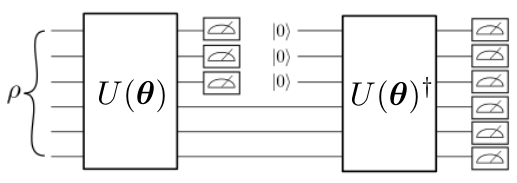
A graphical depiction of a quantum encoder can be seen in the following figure. In a quantum encoder the information contained in some of the input qubits must be discarded after the initial encoding. Then, fresh qubits (here initialized to the |0> state, but one may consider any other easy-to-construct reference state) are prepared and used to implement the final decoding, which is finally compared to the initial state.
The learning task for a quantum autoencoder is to find unitaries which preserve the quantum information of the input through the smaller intermediate latent space. Here, we propose a cost function designed from local operators, possibly avoiding trainability concerns. A figure of merit for the wrong answer when training is simply the total amount of non-zero measurement outcomes on the discarded qubits, which shall be minimized. In order to design the cost function to be local, different outcomes may be penalized by their Hamming distance to the |0> state, which is just the number of symbols that are different in the binary representation. Notice that this cost function has a value of zero if and only if the compression is successfully completed. Note as well that it is defined in terms of local observables and therefore, it does not suffer, for circuits of depth O(log n), from the problem of exponentially vanishing gradients.
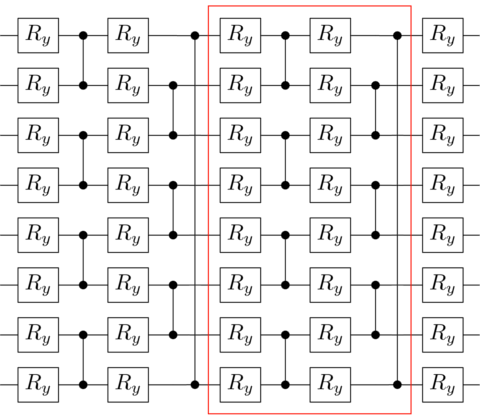
To implement the quantum autoencoder model on a quantum computer we must define the form of the parametrized unitary, decomposing it into a quantum circuit suitable for optimization. In the following figure we depict the ansatz that we have considered. It consists of layers composed of CZ gates acting on alternating pairs of neighboring qubits which are preceded by Ry qubit rotations. After implementing the layered ansatz, a final layer of Ry qubit gates is applied. Finally, measurements on the desired discarded qubits have to be performed for the training. In this example, we encode the Ising model for different λ.
How to run an example?#
To run a particular instance of the problem we have to set up the initial arguments:
nqubits(int): number of quantum bits.layers(int): number of ansatz layers.compress(int): number of compressed/discarded qubits.lambdas(list or array): different λ on the Ising model to consider for the training.
As an example, in order to compress 2 qubits on an initial quantum state with 6 qubits, and using 3 layers, you should execute the following command:
python main.py --nqubits 6 --layers 3 --compress 2 --lambdas [0.9, 0.95, 1.0, 1.05, 1.10]