Adiabatic evolution for solving an Exact Cover problem#
Code at: https://github.com/qiboteam/qibo/tree/master/examples/adiabatic3sat
Introduction#
Adiabatic quantum computation aims to reach the ground state of a problem Hamiltonian encoding the solution of a hard problem, by adiabatically evolving a system from the ground state of a known, easy to prepare, Hamiltonian to the problem Hamiltonian.
An Exact Cover instance of a 3SAT problem is characterized by a set of clauses containing 3 bits that are considered satisfied if one of them is in position 1, while the other remain at 0. The solution of this instance is bitstring that fulfils all the clauses at the same time.
Adiabatic evolution#
Adiabatic computation deals with finding the ground state of a Hamiltonian that encodes the solution of a computational problem. This has to be mapped to the time dependent Hamiltonian in the form
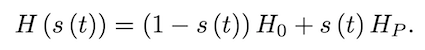
where H_0 and H_p are the initial and problem Hamiltonian respectively, and s(t) defines the schedule that the adiabatic evolution follows. How fast this evolution can be performed depends on the minimum gap energy of the system during the evolution, that is the difference of energy between the ground state and the first excited state along the schedule. The smaller the gap energy the slower the evolution has to be.
The initial Hamiltonian used in this example is the following,
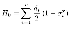
which has a ground state of the equal superposition of all possible computational states.
As for the problem Hamiltonian that encodes the solution of an Exact cover problem, first we define the operator
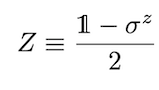
that can be used to create a Hamiltonian with a ground state when the Exact Cover clause is satisfied. This clause Hamiltonian reads
where the indices i, j, k represent the three different qubits that the particular clause addresses. After this is defined, the problem Hamiltonian only needs to add up all clause Hamiltonians, so that the only state that remains at 0 energy will be the one that fulfils at the same time
How to run the example?#
Run the file main.py from the console to perform an adiabatic evolution for an instance of 8 qubits.
The program supports the following basic arguments:
--nqubits(int) allows for instances with different number of qubits (default=8).--instance(int) choose instance to use (default=1).--T(float) set the total time of the adiabatic evolution (default=10).--dt(float) set the interval of the calculations over the adiabatic evolution (default=1e-2).--solver(str) set the type of solver for the evolution (default=’exp’).--plotadd this modifier to output energy and gap plots during the evolution. Capped under 14 qubits due to memory.--trotteradd this modifier to perform the trotterization of the Hamiltonian.
The program returns:
The most common solution found after the evolution.
The probability of the most common solution.
{}_qubits_energy.pngplots detailing the evolution of the lowest two eigenvalues for {} qubits. (if enabled){}_qubits_gap.pngplots detailing the evolution of the gap energy for {} qubits. (if enabled)
Initially supported number of qubits are [4, 8, 10, 12, 14, 16, 18, 20, 22, 24, 26, 28, 30], with 10 different instances for qubits 8 and up.
The main.py script uses linear scheduling for the adiabatic evolution by
default. The user may switch the scheduling function to a polynomial of
arbitrary order by passing the following argument:
--params(str) list of float values separated with commas (,) that define the coefficients of the polynomial scheduling. The polynomial is constructed so that it satisfies s(0)=0 and s(T)=T by definition.
It is also possible to optimize the polynomial coefficients using the following arguments:
--method(str) optimization method to use. See the Qibo optimizer documentation for more details on the available optimization methods.--maxiter(int) maximum number of optimization iterations
When an optimization method is given then the given --params are used as the
initial guess for the variational parameters. If no --params are given linear
scheduling is used and only the final time T is optimized.
The functions used in this example, including problem hamiltonian creation are
included in functions.py.
Create your own instances#
An example of an instance for 4 qubits reads:
 4 3 1
0 1 0 0
 1 2 3
 2 3 4
 1 2 4
The first line includes:
number of qubits
number of clauses
number of 1’s in the solution
The second line is the solution of the instance.
The following lines correspond to the three qubits present in each clause.
Should the solution not be known, leave an empty line in place of the solution as well as remove the number of 1’s in the solution.
Optimization example#
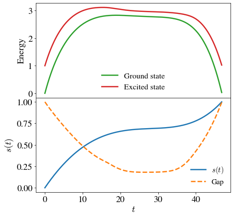
For demonstration we use main.py to optimize a 3SAT instance with N=10 qubits.
We use a fourth order polynomial as the ansatz for the scheduling and after
optimizing the coefficients and the total evolution time T using
scipys BFGS method
we find that the optimal values are:
-3.96837267,0.6582704,1.29674208 and T=46.85073995.
Executing the script for these parameters we find the correct bitstring
solution 0110000101 to the 3SAT problem with probability 99%.
In the plot that follows we show the ground and excited state energies for the adiabatic evolution Hamiltonian, as well as the difference between them (gap) and the final form of the optimized scheduling function. We observe that in agreement with what we expect from theory the scheduling is “slower” at the area where the gap is minimum.
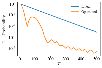
Below we plot the probability to measure the correct solution from the final state of the evolution as a function of the total evolution time T. We find that when using the optimized scheduling (fourth order polynomial) the probability reaches 99% within T=50, while for the default linear scheduling T=400 is required to reach the same probability.