Quantum Convolutional Neural Network Classifier#
Code at: https://github.com/qiboteam/qibo/tree/main/examples/qcnn_classifier. Please note that scikit-learn is needed to visualize the results.
Problem overview#
This tutorial implements a simple Quantum Convolutional Neural Network (QCNN), which is a translationally invariant algorithm analogous to the classical convolutional neural network. This example demonstrates the use of the QCNN as a quantum classifier, which attempts to classify ground states of a translationally invariant quantum system, the transverse field Ising model, based on whether they are in the ordered or disordered phase. The (randomized) statevector data provided are those of a 4-qubit system. Accompanying each state is a label: +1 (disordered phase) or -1 (ordered phase).
Through the sequential reduction of entanglement, this network is able to perform classification from the final measurement of a single qubit.
Workflow of QCNN model: 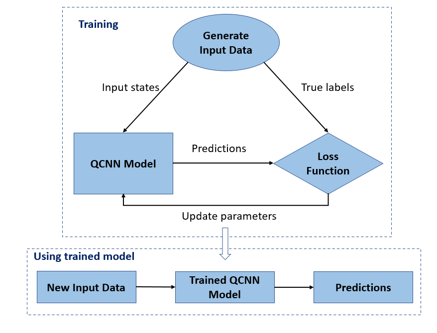
Schematic of QCNN model: 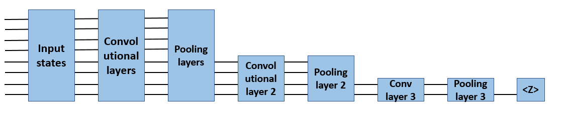
Convolutional layer for 4 qubits as an example: 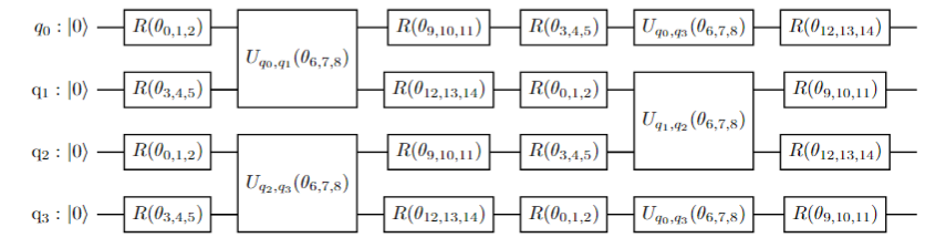
Pooling layer for 4 qubits as an example: 
where in the above, \(R(\theta_{i,j,k}) = RZ(\theta_k) RY(\theta_j) RX(\theta_i)\): 
\(U_{q_a, q_b}(\theta_{i,j,k}) = RXX(\theta_k) RYY(\theta_j) RZZ(\theta_i)\) is a two-qubit gate acting on qubits \(q_a\) and \(q_b\): 
and \(R^{\dagger}(\theta_{i,j,k}) = RX(-\theta_i) RY(-\theta_j) RZ(-\theta_k)\): 
How to use the QCNN class#
For more details on the QuantumCNN class, please refer to the documentation. Here we recall some of the necessary arguments when instantiating a QuantumCNN object: - nqubits (int): number of quantum bits. It should be larger than 2 for the model to make sense. - nlayers (int): number of layers of the QCNN variational ansatz. - nclasses (int): number of classes of the training set (default=2). - params: list to initialise the variational parameters (default=None).
After creating the object, one can proceed to train the model. For this, the QuantumCNN.minimize method can be used with the following arguments (refer to the documentation for more details)” - init_theta: list or numpy.array with the angles to be used in the circuit - data: the training data - labels: numpy.array containing the labels for the training data - nshots (int):number of runs of the circuit during the sampling process (default=10000) - method (string): str
‘classical optimizer for the minimization’. All methods from scipy.optimize.minmize are suported (default=‘Powell’).
QCNN Demo#
Include necessary packages:
[4]:
import random

import numpy as np
from sklearn import metrics

import qibo
from qibo.models.qcnn import QuantumCNN

qibo.set_backend("numpy")
[Qibo 0.1.13|INFO|2023-05-15 17:25:59]: Using numpy backend on /CPU:0
Load the provided data (ground states of 4-qubit TFIM in data folder) and labels:
[5]:
data = np.load("nqubits_4_data_shuffled_no0.npy")
labels = np.load("nqubits_4_labels_shuffled_no0.npy")
labels = np.transpose(np.array([labels]))  # restructure to required array format
Structure of data and labels are like:
[6]:
data[-2:]
[6]:
array([[0.52745364+0.j, 0.19856967+0.j, 0.19856967+0.j, 0.16507377+0.j,
        0.19856967+0.j, 0.09784837+0.j, 0.16507377+0.j, 0.19856967+0.j,
        0.19856967+0.j, 0.16507377+0.j, 0.09784837+0.j, 0.19856967+0.j,
        0.16507377+0.j, 0.19856967+0.j, 0.19856967+0.j, 0.52745364+0.j],
       [0.67109214+0.j, 0.10384038+0.j, 0.10384038+0.j, 0.05351362+0.j,
        0.10384038+0.j, 0.02786792+0.j, 0.05351362+0.j, 0.10384038+0.j,
        0.10384038+0.j, 0.05351362+0.j, 0.02786792+0.j, 0.10384038+0.j,
        0.05351362+0.j, 0.10384038+0.j, 0.10384038+0.j, 0.67109214+0.j]])
[7]:
labels[-2:]
[7]:
array([[ 1.],
       [-1.]])
Split the data into training/test set in the ratio 60:40
[8]:
split_ind = int(len(data) * 0.6)
train_data = data[:split_ind]
test_data = data[split_ind:]

train_labels = labels[:split_ind]
test_labels = labels[split_ind:]
Initialize the QuantumCNN class:
[9]:
test = QuantumCNN(nqubits=4, nlayers=1, nclasses=2)
testcircuit = test._circuit
testcircuit.draw()
q0:     ─RX─RY─RZ─RZZ─RYY─RXX─RX─RY─RZ──────────────────────────────────────── ...
q1:     ─RX─RY─RZ─RZZ─RYY─RXX─RX─RY─RZ─────────────RX─RY─RZ──────────RZZ─RYY─R ...
q2:     ──────────────────────RX─RY─RZ─RZZ─RYY─RXX─RX─RY─RZ─RX─RY─RZ─RZZ─RYY─R ...
q3:     ──────────────────────RX─RY─RZ─RZZ─RYY─RXX─RX─RY─RZ─────────────────── ...

q0: ... ───RX─RY─RZ─RZZ─RYY─RXX─RX─RY─RZ─RX─RY─RZ─o───────────────────────
q1: ... XX─RX─RY─RZ─|───|───|─────────────────────|─RX─RY─RZ─o────────────
q2: ... XX─RX─RY─RZ─|───|───|───RX─RY─RZ──────────X─RZ─RY─RX─|────────────
q3: ... ───RX─RY─RZ─RZZ─RYY─RXX─RX─RY─RZ────────────RX─RY─RZ─X─RZ─RY─RX─M─
draw() is used to visualize the pre-constructed circuit based on input parameters for class initialization.
Initialize model parameters:
[ ]:
testbias = np.zeros(test.measured_qubits)
testangles = [random.uniform(0, 2 * np.pi) for _ in range(21 * 2)]
init_theta = np.concatenate((testbias, testangles))
Train model with optimize parameters (automatically updates model with optimized paramters at the end of training):
[ ]:
result = test.minimize(
    init_theta, data=train_data, labels=labels, nshots=10000, method="Powell"
)
Alternatively, update model with optimized parameters from previous training:
[11]:
saved_result_60 = (
    0.2026119742575817,
    np.array(
        [
            -0.06559061,
            3.62881221,
            2.39850148,
            3.02493711,
            0.91498683,
            3.25517842,
            0.0759049,
            3.46049453,
            3.04395784,
            1.55681424,
            2.3665245,
            0.40291846,
            5.67310744,
            2.27615444,
            5.23403537,
            0.46053411,
            0.69228362,
            2.2308165,
            0.53323661,
            4.52157388,
            5.31194656,
            18.23511858,
            -1.90754635,
            14.30577217,
            10.75135972,
            19.16001316,
            12.27582746,
            7.47476354,
            23.38129141,
            60.29771502,
            10.02946377,
            17.83945879,
            15.22732248,
            12.34666584,
            1.52634649,
            1.90621517,
            12.71554053,
            -13.56379057,
            34.04591253,
            -11.56450878,
            10.95038782,
            3.30640208,
            9.67270071,
        ]
    ),
)

test.set_circuit_params(angles=saved_result_60[1], has_bias=True)
Generate predictions from optimized model:
[12]:
predictions = []
for n in range(len(test_data)):
    predictions.append(test.predict(test_data[n], nshots=10000)[0])
Visualize results via confusion matrix and accuracy:
[14]:
actual = [np.sign(test_labels) for test_labels in test_labels]
predicted = [np.sign(prediction) for prediction in predictions]

confusion_matrix = metrics.confusion_matrix(actual, predicted)

cm_display = metrics.ConfusionMatrixDisplay(
    confusion_matrix=confusion_matrix, display_labels=[1, -1]
)

cm_display.plot()
[14]:
<sklearn.metrics._plot.confusion_matrix.ConfusionMatrixDisplay at 0x7efd85b82200>
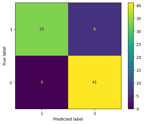
[15]:
test.Accuracy(test_labels, predictions)
[15]:
0.925