Calibration of CNOT gate using Cross-Resonance

It is possible to generate an interaction between two superconducting qubits without requiring flux tunability, through a mechanism known as Cross Resonance (CR). This mechanism relies only on microwave drive pulses. Moreover, not using flux lines, results in a reduction of the number of fridge lines and allows to ignore all problems related to flux noise.

The cross resonance effect was first proposed [21] in and later independently discovered in [11, 26].

The CR effect can be showed by starting with the Hamiltonian of a two-qubit system with a drive term on the first qubit [18]

\[H = b_1^\dagger b_1 \omega_1 + \frac{\alpha_1}{2} b_1^\dagger b_1^\dagger b_1 b_1 + b_2^\dagger b_2 \omega_2 + \frac{\alpha_2}{2} b_2^\dagger b_2^\dagger b_2 b_2 + g (b_1 b_2^\dagger + b_1^\dagger b_2) + \Omega(t) (b_1 + b_1^\dagger)\]

If we are in a dispersive regime (i.e. \(|\omega_1 - \omega_2| \gg g\)), through a Schrieffer-Wolff transformation we can obtain the effective Hamiltonian:

\[H_\text{eff} = - \frac{\tilde{\omega_1}}{2} \sigma_1^z - \frac{\tilde{\omega_2}}{2} \sigma_2^z + \frac{\zeta}{4} \sigma_1^z \sigma_2^z + \Omega(t) \Big[ \sigma_1^x + \nu \sigma_2^x + \mu \sigma_1^z \sigma_2^x\Big]\]

where \(\zeta\) is the ZZ coupling, \(\nu\) is quantum crosstalk factor and \(\mu\) is the cross-resonance factor. From the equation above we can see that by driving the first qubit at the frequency of the second qubit .

By tuning the amplitude and the duration of this drive pulse it is possible to calibrate a \(RZX\) rotation to rotate exactly by \(- \pi/2\). This is done because starting from a \(ZX_{frac{\pi}{2}}\) we can obtain a CNOT gate using single qubit rotations.

\[\text{CNOT} = \text{R}_\text{ZX}(-\pi/2) \text{R}_\text{IX}(\pi/2) \text{R}_\text{ZI}(\pi/2)\]

In Qibocal we provide protocols to calibrate CR pulses.

Sweeping the duration of the CR pulse

In a first experiment we can sweep the duration of the CR pulse and measure both the target and control qubit. The measurement is performed while preparing the control qubit in state \(\ket{0}\) and \(\ket{1}\).

Parameters

Example

A possible runcard to launch the experiment could be the following:

- id: CR length
  operation: cross_resonance_length
  parameters:
    targets: [[0,1]]
    pulse_duration_start: 10
    pulse_duration_end: 200
    pulse_duration_step: 10
    flux_pulse_amplitude: 0.1
    nshots: 2000
    relaxation_time: 50000

The expected output is the following:

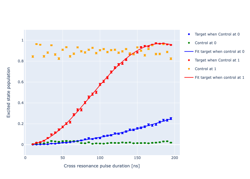
Post-processing

The probability of the target qubit is fitted in both cases to a dumped cosine functions. It is possible to extract the effective coupling as

\[\text{J}_\text{eff}/ 2 \pi = \frac{f^{\pi}_\text{Rabi} - f_\text{Rabi}}{2}\]

where \(f^{\pi}_\text{Rabi}\) and \(f_\text{Rabi}\) are the frequencies of the fitted Rabi oscillations on the target qubit.

Sweeping amplitude of the CR pulse

Similarly it is possible to sweep the amplitude of the CR pulse and measure both the target and control qubit.

Parameters

Example

A possible runcard to launch the experiment could be the following:

- id: CR amplitude
  operation: cross_resonance_amplitude
  parameters:
    targets: [[0,1]]
    max_amp: 0.05
    min_amp: 0.01
    step_amp: 0.005
    pulse_duration: 100
    nshots: 2000
    relaxation_time: 50000

The expected output is the following:

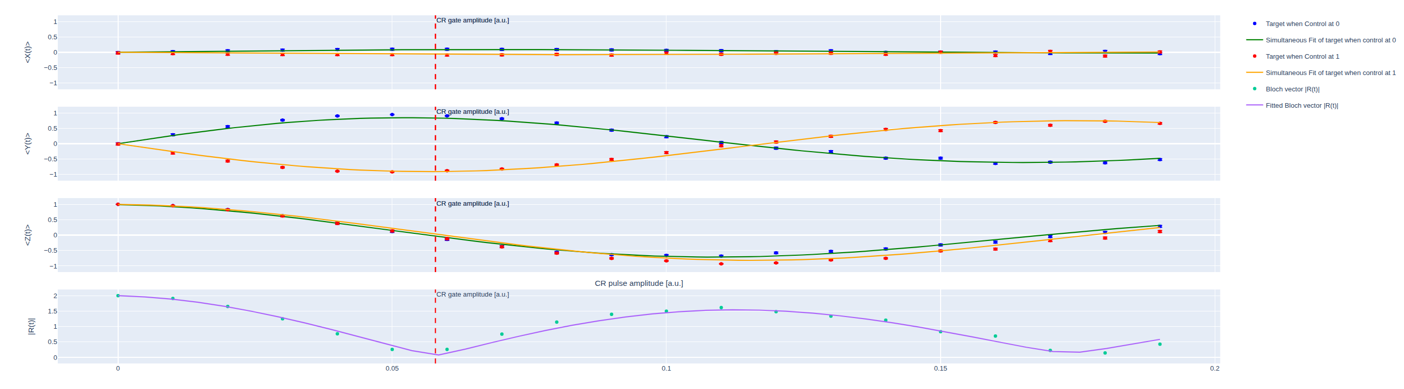
Post-processing

The probability of the target qubit is fitted in both cases to a cosine function.

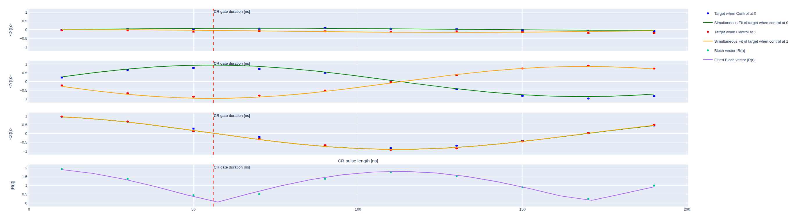
Hamiltonian Tomography measurement

Although from the two previous experiments it is possible to perform an initial calibration of the CR gate, by performing a state tomography on the target qubit it is possible to reconstruct the effective Hamiltonian of the system [17]:

\[H_\text{eff} = \frac{\nu_\text{ZX}}{2} \text{ZX} + \frac{\nu_\text{ZY}}{2} \text{ZY} + \frac{\nu_\text{ZZ}}{2} \text{ZZ} + \frac{\nu_\text{IX}}{2} \text{IX} + \frac{\nu_\text{IY}}{2} \text{IY} + \frac{\nu_\text{IZ}}{2} \text{IZ}\]

In particular, by sweeping the duration of the CR pulse and measuring the expectation values of the target qubit \(\langle X \rangle\), \(\langle Y \rangle\) and \(\langle Z \rangle\) when the control qubit is prepared in \(\ket{0}\) and \(\ket{1}\) we can compute all terms in the effective Hamiltonian following the procedure in [17].

Parameters

Example

A possible runcard to launch the experiment could be the following:

- id: Hamiltonian tomography CR
  operation: cross_resonance_amplitude
  parameters:
    targets: [[0,1]]
    nshots: 2000
    pulse_amplitude: 0.1
    pulse_duration_end: 400
    pulse_duration_start: 10
    pulse_duration_step: 20

The expected output is the following:

Requirements

To run these experiments single qubit gates for both target and control qubit needs to be calibrated.