Basic examples
In this section we are going to explain briefly how to perform the calibration of single qubit devices.
Dummy guide for single qubit calibration
Not flux tunable qubits
The calibration of a not flux-tunable superconducting chip includes the following steps:
- Resonator characterization:
Probing the resonator at high power
Estimating the readout amplitude through a punchout
Finding the dressed resonator frequency
- Qubit characterization
Finding the qubit frequency
Calibrating the \(\pi\) pulse
Building classification model for \(\ket{0}\) and \(\ket{1}\)
We are going to explain how to use qibocal to address each step of the calibration.
Resonator characterization
Each qubit is coupled to a resonator to perform the measurement. The resonator is characterized by a bare frequency that can be extracted by running a resonator spectroscopy at high power. To perform this experiment with qibocal it is sufficient to write the following action:
- id: resonator_spectroscopy high power

  operation: resonator_spectroscopy
  parameters:
      freq_width: 60_000_000
      freq_step: 200_000
      amplitude: 0.6
      power_level: high
      nshots: 1024
      relaxation_time: 100000
In order to learn how to run this action using Qibocal you can a look at this tutorial.
The choice of the parameters is arbitrary. In this specific case the user should make sure to specify an amplitude value sufficiently large.
It is then possible to visualize a report included in the output folder.
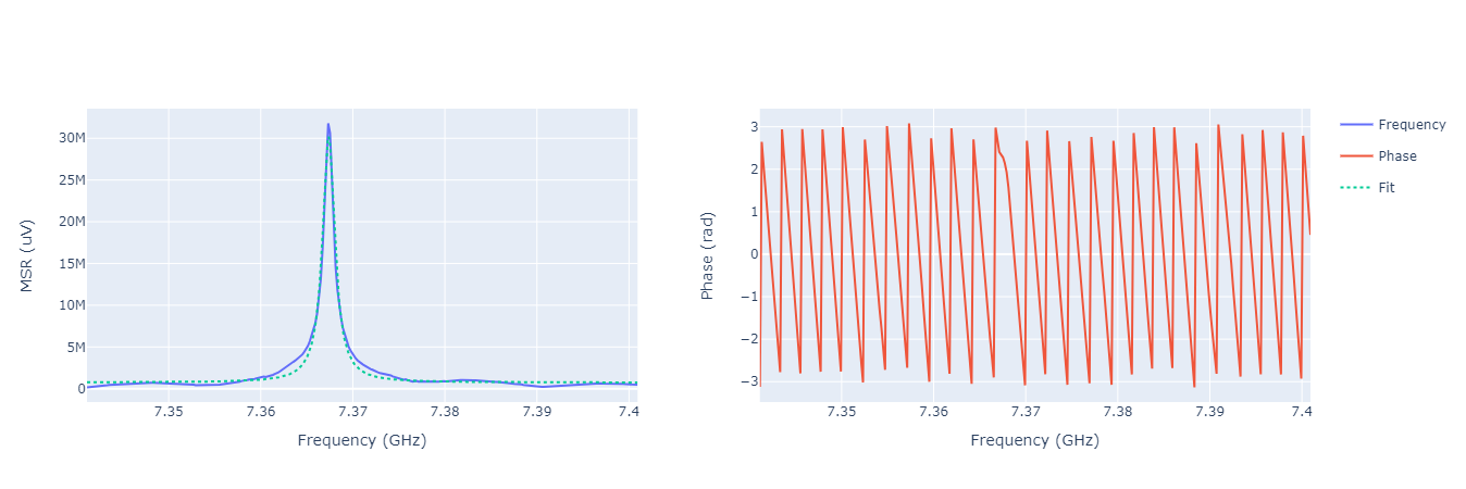
The expected signal is a lorentzian centered around the bare frequency of the resonator.
At lower power, the resonator will be coupled to the qubit in the dispersive regime. The coupling manifests itself in a shift of the energy levels. In order to check at which power we observe this shift it is possible to run a resonator punchout using the following punchout.yaml runcard.
- id: resonator punchout

  operation: resonator_punchout
  parameters:
      freq_width: 40_000_000
      freq_step: 500_000
      amplitude: 0.03
      min_amp: 0.1
      max_amp: 2.4
      step_amp: 0.3
      nshots: 2048
      relaxation_time: 5000
Which corresponds to a 2D scan in amplitude and readout frequency. After executing the experiment with the previous syntax we should see something like this.
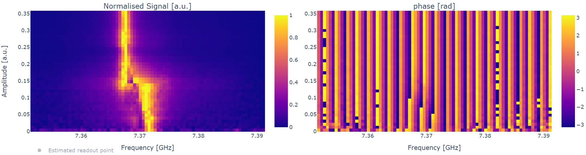
The image above shows that below 0.15 amplitude the frequency of the resonator shifted as expected.
Finally, now that we have a reasonable guess for the readout amplitude we can eventually run again a resonator spectroscopy putting the correct readout amplitude value.
Here is an example of a runcard.
- id: resonator_spectroscopy low power

  operation: resonator_spectroscopy
  parameters:
      freq_width: 60_000_000
      freq_step: 200_000
      amplitude: 0.03
      power_level: low
      nshots: 1024
      relaxation_time: 100000
Note that in this case we changed the power_level entry from
high to low, this keyword is used by qibocal to upgrade
correctly the QPU parameters depending on the power regime.
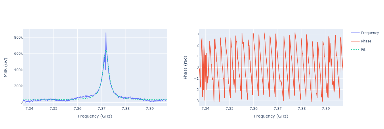
Note
Depending on the resonator type the resonator frequency might appear as a deep or a peak.
Qubit characterization
After having a rough estimate on the readout frequency and the readout amplitude, we can start to characterize the qubit.
The qubit transition frequency \(\omega_{01}\),the frequency of the transition between state \(\ket{0}\) and state \(\ket{1}\), is determined using a dispersive spectroscopy measurement.
Here is an example runcard:
- id: qubit spectroscopy 01

  operation: qubit_spectroscopy
  parameters:
      drive_amplitude: 0.5
      drive_duration: 4000
      freq_width: 100_000_000
      freq_step: 100_000
      nshots: 1024
      relaxation_time: 5000
For this particular experiment it is recommended to use
a drive_duration large compared to the coherence time of
the qubit. Currenty the coherence time for transmon qubits
if of the order of \(10^3 - 10^6\) ns.
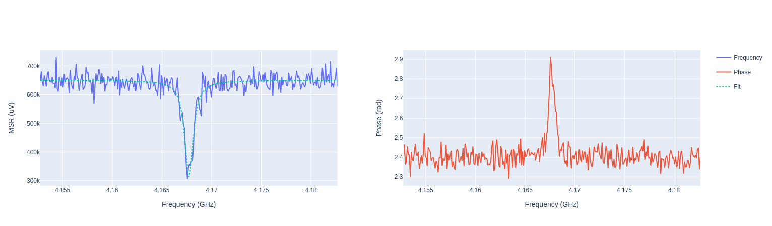
Similarly to the resonator, we expect a lorentzian peak around \(\omega_{01}\) which will be our drive frequency.
Note
By using high values of drive_amplitude it might be possible to see
another peak which corresponds to \(\omega_{02}/2\).
Note
Depending on the resonator type the qubit frequency might appear as a deep or a peak.
Note
If the qubit is flux-tunable make sure to have a look at this section.
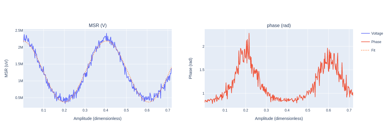
The missing step required to perform a transition between state \(\ket{0}\) and state \(\ket{1}\) is to calibrate the amplitude of the drive pulse, also known as \(\pi\) pulse.
Such amplitude is estimated through a Rabi experiment, which can be executed in qibocal through the following runcard:
- id: rabi

  operation: rabi_amplitude_signal
  parameters:
      min_amp: 0
      max_amp: 1.1
      step_amp: 0.1
      pulse_length: 40
      relaxation_time: 100_000
      nshots: 1024
In this particular case we are fixing the duration of the pulse to be 40 ns and we perform a sweep in the drive amplitude to find the correct value. The \(\pi\) corresponds to first half period of the oscillation.
Classification model
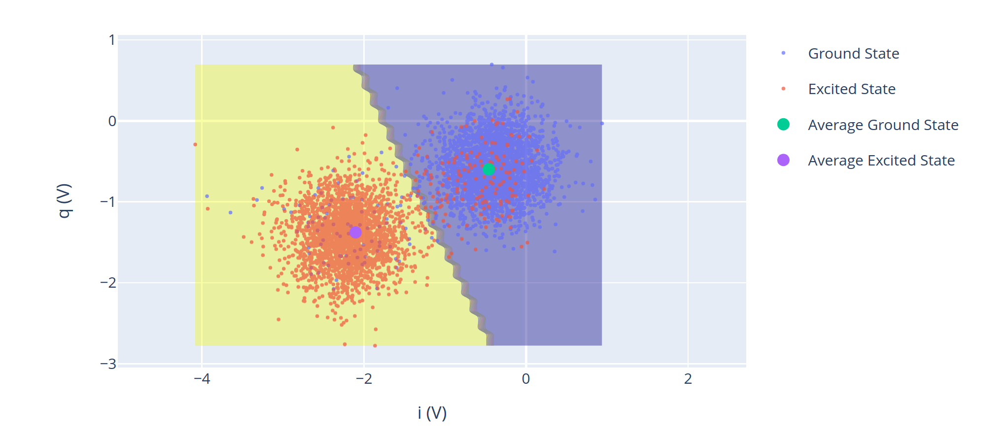
Now that we are able to produce \(\ket{0}\) and \(\ket{1}\) we need to build a model that will discriminate between these two states, also known as classifier. Qibocal provides several classifiers of different complexities including Machine Learning based ones.
The simplest model can be trained by running the following experiment:
- id: single shot classification 1

  operation: single_shot_classification
  parameters:
      nshots: 5000
The expected results are two separated clouds in the IQ plane.
Flux tunable qubits
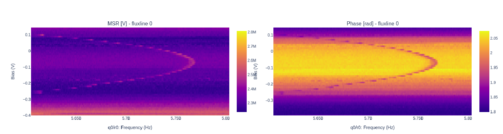
When dealing with flux tunable qubits it is important to also study how the qubit reacts when changing the magnetic flux. From the theory we know that by modifying the flux the qubit frequency will be modified.
Usually we should characterize the qubit in the flux range where it is most insensitive to a
a change in flux, also know as sweetspot.
We can study the flux dependence of the qubit using the following runcard:
- id: qubit flux dependence

  operation: qubit_flux
  parameters:
      freq_width: 100_000_000
      freq_step: 500_000
      bias_width: 0.20
      bias_step:  0.01
      drive_amplitude: 0.1
      nshots: 1024
      relaxation_time: 20_000
Note
For more complicating applications the optimal point might not be the sweetspot.
Assessing the goodness of the calibration
Several experiments can be performed to estimate the goodness of the calibration.
Measurement of the qubit coherences
The fidelity achievable using a superconducting qubit is limited by the coherence times of the qubit.
To measure the energy decay of a qubit state, also known as \(\\T_1\). The experiment consists in bringing the qubit to \(\ket{1}\) and then performing a measurement after a waiting time \(\tau\).
Here is the runcard:
- id: t1

  operation: t1
  parameters:
      delay_before_readout_end: 200000
      delay_before_readout_start: 50
      delay_before_readout_step: 1000
      nshots: 1024
      relaxation_time: 300000
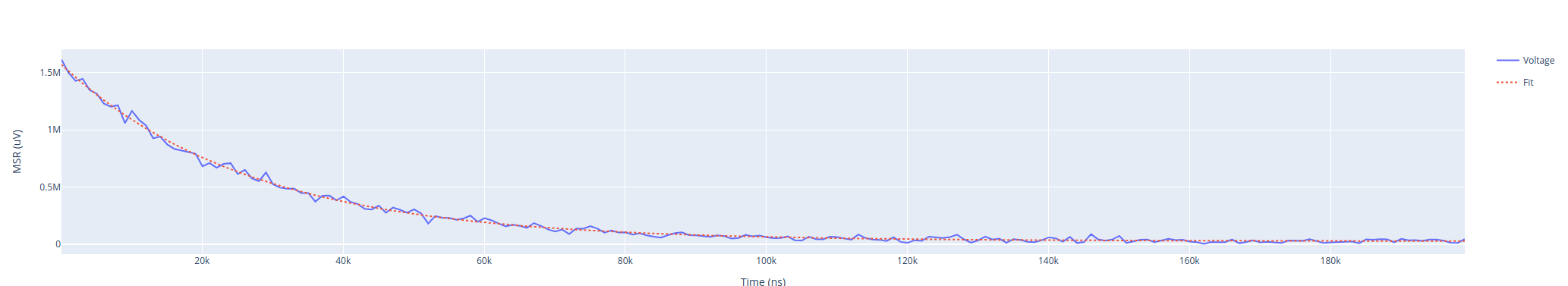
We expect to see an exponential decay whose rate will give us the factor \(\\T_1\).
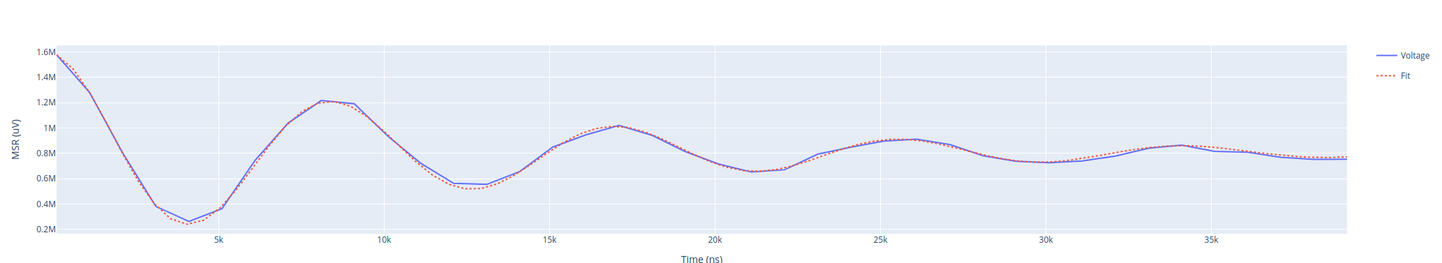
We can also estimate the loss of quantum information due to the loss in the knowledge of the phase of a quantum state. Such parameter is denoted with \(\\T_2\) and can be estimated through a Ramsey experiment.
- id: ramsey detuned

  operation: ramsey
  parameters:
      delay_between_pulses_end: 40000
      delay_between_pulses_start: 100
      delay_between_pulses_step: 1000
      n_osc: 0
      nshots: 4096
      relaxation_time: 200000
Fidelities
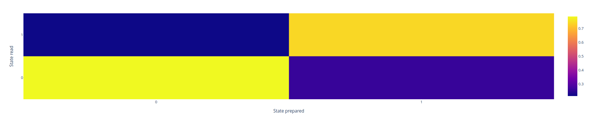
We can estimate the assignment fidelity \(\\\mathcal{F}\) which is defined as [9]
where \(P(m=X|\ket{Y}_i)\) is the probability of measuring \(\ket{X}\) after having prepared \(\ket{Y}\).
- id: readout characterization

  operation: readout_characterization
  parameters:
      nshots: 5000
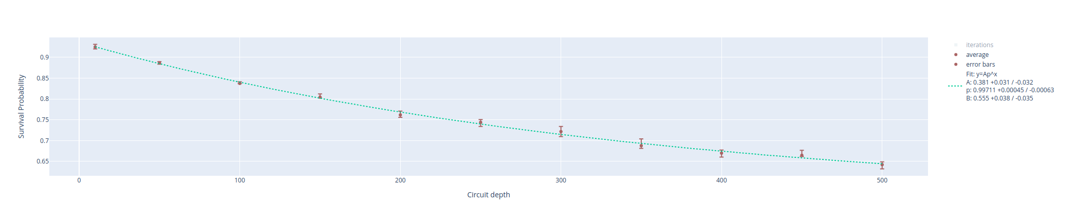
In order to estimate a gate-fidelity which is unaffected by State Preparation And Measurement (SPAM) errors it is possible to run a standard randomized benchmarking.
- id: standard rb
  operation: standard_rb
  parameters:
      depths: [10, 50, 100, 150, 200, 250, 300, 350, 400, 450, 500]
      niter: 256
      nshots: 128