Readout optimization¶

Qibocal provides different protocols to improve the readout pulse parameters by optimizing the assignment fidelity.

Readout Amplitude Optimization¶

The readout amplitude protocol improves the readout amplitude by optimizing the assignment fidelity.

Parameters¶

class qibocal.protocols.readout.amplitude_optimization.ReadoutAmplitudeParameters(amplitude_range: tuple[float, float, float] | tuple[Literal['linspace'], float, float, int] | tuple[Literal['window'], float, float, float] | tuple[Literal['linwindow'], float, float, int] | tuple[Literal['center'], float, float] | tuple[Literal['lincenter'], float, int] | tuple[Literal['asym'], tuple[float, float], float] | tuple[Literal['linasym'], tuple[float, float], int], save_iq: bool = False)[source]

ReadoutAmplitude runcard inputs.

amplitude_range: tuple[float, float, float] | tuple[Literal['linspace'], float, float, int] | tuple[Literal['window'], float, float, float] | tuple[Literal['linwindow'], float, float, int] | tuple[Literal['center'], float, float] | tuple[Literal['lincenter'], float, int] | tuple[Literal['asym'], tuple[float, float], float] | tuple[Literal['linasym'], tuple[float, float], int]

Amplitude RangeLike object.

For further information, see qibocal.protocols.utils.RangeLike.

save_iq: bool = False: Whether to save the IQ data during the acquisition.

nshots: int: Number of executions on hardware.

relaxation_time: float: Wait time for the qubit to decohere back to the ground state.

Example¶

It follows an example runcard of the readout amplitude routine with the plot generated in the report.

- id: ro_amplitude
  operation: ro_amplitude
  parameters:
      amplitude_range: [0.001, 0.005, 0.0005]

As shown in the picture below, the protocol sweeps the readout amplitude and evaluates the errors probability.

Readout Frequency Optimization¶

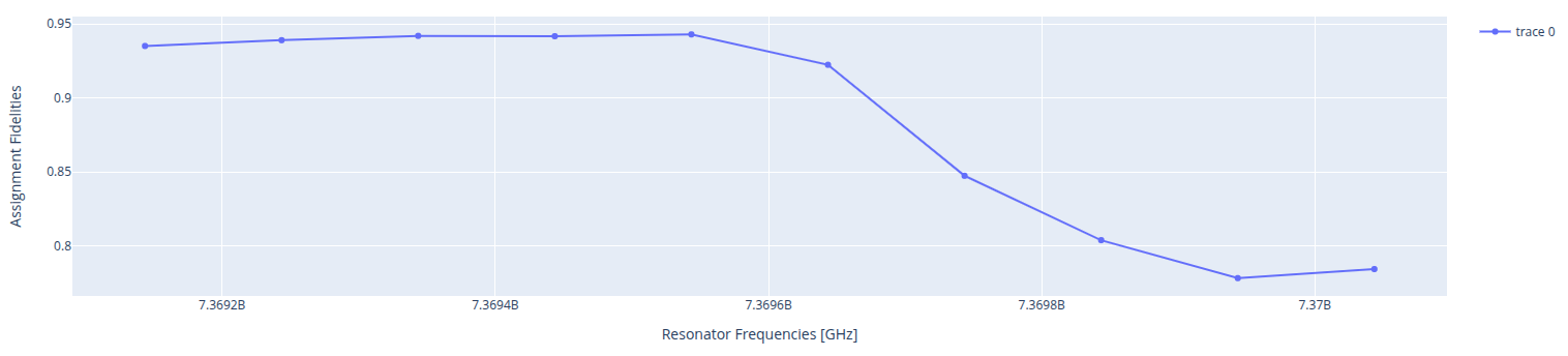
The readout frequency protocol performs a sweep of the readout frequency to maximize assignment fidelity.

Parameters¶

class qibocal.protocols.readout.frequency_optimization.ReadoutFrequencyParameters(frequency_range: tuple[float, float, float] | tuple[Literal['linspace'], float, float, int] | tuple[Literal['window'], float, float, float] | tuple[Literal['linwindow'], float, float, int] | tuple[Literal['center'], float, float] | tuple[Literal['lincenter'], float, int] | tuple[Literal['asym'], tuple[float, float], float] | tuple[Literal['linasym'], tuple[float, float], int], save_iq: bool = False)[source]

Optimization RO frequency inputs.

frequency_range: tuple[float, float, float] | tuple[Literal['linspace'], float, float, int] | tuple[Literal['window'], float, float, float] | tuple[Literal['linwindow'], float, float, int] | tuple[Literal['center'], float, float] | tuple[Literal['lincenter'], float, int] | tuple[Literal['asym'], tuple[float, float], float] | tuple[Literal['linasym'], tuple[float, float], int]

Frequency RangeLike object.

For further information, see qibocal.protocols.utils.RangeLike.

save_iq: bool = False: Whether to save the IQ data during the acquisition.

nshots: int: Number of executions on hardware.

relaxation_time: float: Wait time for the qubit to decohere back to the ground state.

Example¶

In the following we show a possible runcard for the optimization of the readout frequency together with expected output plot.

- id: ro_frequency
  operation: ro_frequency
  parameters:
    freq_range: ['center', 1_000_000, 100_000]

../../_images/frequency_optimization.png

Readout Amplitude-Frequency Simultaneous Optimization¶

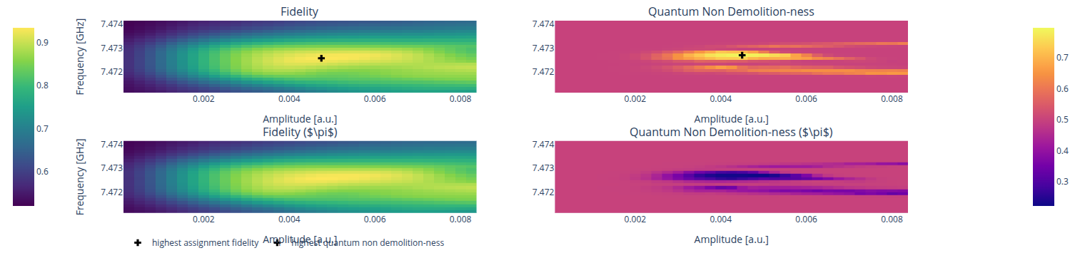
In addition to this metric, the protocol also computes the quantum non-demolition-ness (QND) of the measurement, which serves to evaluate measurement-induced state disturbance. To capture leakage outside the computational basis the protocol includes the computation of QND with an additional \(\pi\) pulse. Readout parameters are then updated based on the configuration that yields the highest assignment fidelity.

Parameters¶

Example¶

A possible runcard for the resonator optimization protocol could be:

- id: ro_amplitude_frequency
  operation: ro_amplitude_frequency
  parameters:
    freq_range: ['center', 3_000_000, 125_000]
    amplitude_range: [0.00025, 0.0085, 0.00025]
    delay: 1000

The plot generated by the report should be similar to the following one:

../../_images/resonator_optimization.png