Variational Quantum Linear Solver

This tutorial aims to implement the Variational Quantum Linear Solver(VQLS) algorithm proposed by Carlos Bravo-Prieto et al.

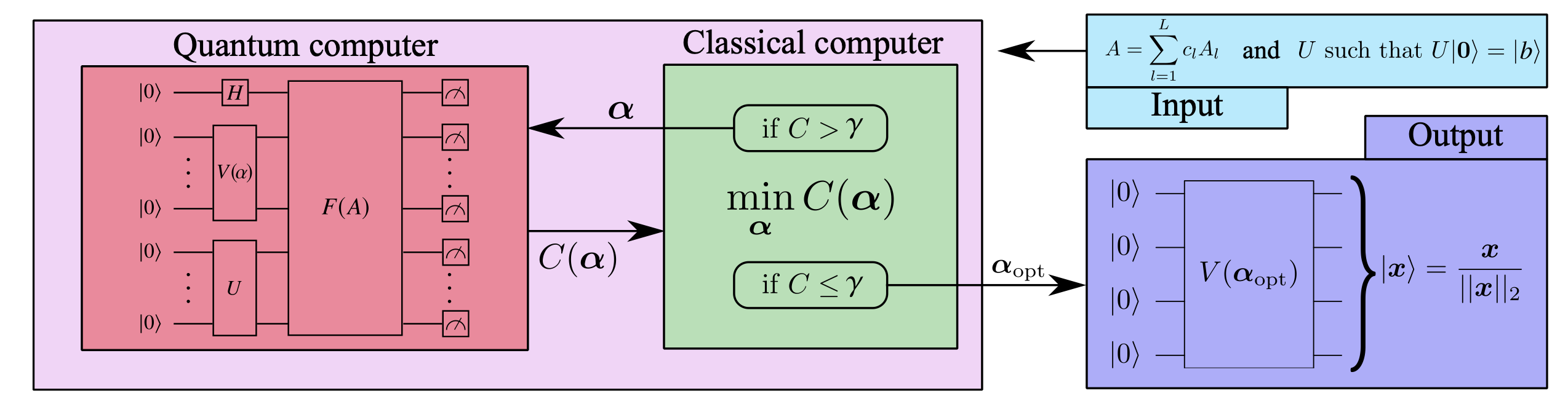
The algorithm takes as input a matrix A written as a linear combination of unitaries AL and a short-depth quantum circuit U which prepares the state |b⟩, and produces a quantum state |x⟩ that is approximately proportional to the solution of the linear system Ax= b.

Imports

import numpy as np
import matplotlib.pyplot as plt

import torch
import torch.optim as optim

from qibo import (
    Circuit,
    gates,
    set_backend,
)

from qiboml.models.decoding import VariationalQuantumLinearSolver
from qiboml.interfaces.pytorch import QuantumModel

Define Hyperparameters

Setting backend to “pytorch” enables automatic differentiation of quantum circuits using PyTorch. This allows us to use the ADAM optimizer when optimizing the circuit parameters.

# Set backend
set_backend("qiboml", platform="pytorch")

# Hyper-parameters
n_qubits = 3
q_delta  = 0.001
rng_seed = 42
np.random.seed(rng_seed)
weights = q_delta * np.random.randn(n_qubits)

[Qibo 0.2.19|INFO|2025-07-09 09:46:35]: Using qiboml (pytorch) backend on cpu

Representing our Matrix(A) and Target Vector(b)

Matrix A must be represented as a linear combination of unitaries AL

c = np.array([1.0, 0.2, 0.2]) # Coefficients of the linear combination A = c_0 A_0 + c_1 A_1 ...

Id = np.identity(2)
Z = np.array([[1, 0], [0, -1]])
X = np.array([[0, 1], [1, 0]])

A_0 = np.identity(8)
A_1 = np.kron(np.kron(X, Z), Id)
A_2 = np.kron(np.kron(X, Id), Id)

# Linear combination A = c₀A₀ + c₁A₁ + c₂A₂
A_num = c[0] * A_0 + c[1] * A_1 + c[2] * A_2

# Target Vector
b = np.ones(8) / np.sqrt(8)

Initialize Variational Circuit

Variational circuit mapping the ground state \(|0\rangle\) to the ansatz state \(|x\rangle\)

def variational_block(weights):
    variational_ansatz = Circuit(n_qubits)
    for idx in range(n_qubits):
        variational_ansatz.add(gates.H(idx))
    for idx, element in enumerate(weights):
        variational_ansatz.add(gates.RY(idx,element))
    return variational_ansatz

Building Custom Decoder

The parameters should be optimized in order to maximize the overlap between the quantum states \(|\Psi\rangle\) and \(|b\rangle\). To acheive this we define the cost function

\[C_G = 1 - |\langle b | \Psi \rangle|^2\]

which quantifies the infidelity between our two states. When

\[|\langle b | \Psi \rangle|^2 = 1 \quad \text{(perfect overlap)}, \quad C_G = 0.\]

Using the VariationalQuantumLinearSolver class from the QiboML library we are able to generate our desired cost from the output of our variational circuit.

decoder = VariationalQuantumLinearSolver(n_qubits, target_state=b, A = A_num)

Build Model

Use QiboML’s QuantumModel class to build the machine learning model.

# Prepare the test circuit and decoder
circuit = variational_block(weights)

# Build Model
model = QuantumModel(
    decoding=decoder,
    circuit_structure=circuit)

Train Circuit

Use the ADAM optimizer to perform gradient descent on loss landscape and optimize circuit parameters.

optimizer = optim.Adam(model.parameters(), lr=0.05)

# Optimize
for iteration in range(300):
    optimizer.zero_grad()
    cost = model()
    cost.backward()
    optimizer.step()

    if iteration % 20 == 0:
        print(f"Iteration {iteration}: Cost = {cost.item():.6f}")

Iteration 0: Cost = 0.027048
Iteration 20: Cost = 0.000190
Iteration 40: Cost = 0.000196
Iteration 60: Cost = 0.000003
Iteration 80: Cost = 0.000004
Iteration 100: Cost = 0.000001
Iteration 120: Cost = 0.000000
Iteration 140: Cost = 0.000000
Iteration 160: Cost = 0.000000
Iteration 180: Cost = 0.000000
Iteration 200: Cost = 0.000000
Iteration 220: Cost = 0.000000
Iteration 240: Cost = 0.000000
Iteration 260: Cost = 0.000000
Iteration 280: Cost = 0.000000

Final Parameters and Results

optimized_params = model.circuit_parameters.detach().cpu().numpy()
print("Optimized theta values: ", optimized_params)
param_circuit = variational_block(optimized_params)
result = param_circuit.execute()
final_state = result.state().detach().numpy()
print("Final state vector (as amplitudes):")
print(final_state)

Optimized theta values:  [-5.42217344e-09  3.30297394e-01 -8.53152139e-09]
Final state vector (as amplitudes):
[0.29061909+0.j 0.29061909+0.j 0.40686674+0.j 0.40686674+0.j
 0.29061909+0.j 0.29061909+0.j 0.40686674+0.j 0.40686674+0.j]

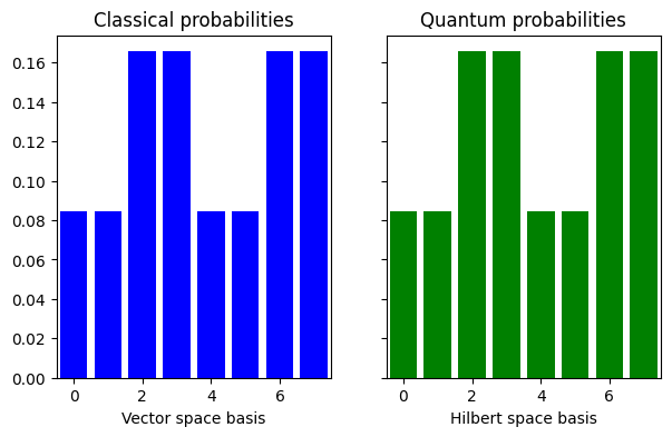
Comparison with Classical Solution

q_probs = np.abs(final_state)**2

A_inv = np.linalg.inv(A_num)
x = np.dot(A_inv, b)

c_probs = (x / np.linalg.norm(x)) ** 2

fig, (ax1, ax2) = plt.subplots(1, 2, figsize=(7, 4), sharey=True)

ax1.bar(np.arange(0, 2 ** n_qubits), c_probs, color="blue")
ax1.set_xlim(-0.5, 2 ** n_qubits - 0.5)
ax1.set_xlabel("Vector space basis")
ax1.set_title("Classical probabilities")

ax2.bar(np.arange(0, 2 ** n_qubits), q_probs, color="green")
ax2.set_xlim(-0.5, 2 ** n_qubits - 0.5)
ax2.set_xlabel("Hilbert space basis")
ax2.set_title("Quantum probabilities")

plt.show()