Variational Quantum Eigensolver

A variational quantum eigensolver is a variational quantum algorithm where a parametrized quantum circuit is trained to prepare the ground state of a target Hamiltonian See A. Peruzzo et al. - 2013.

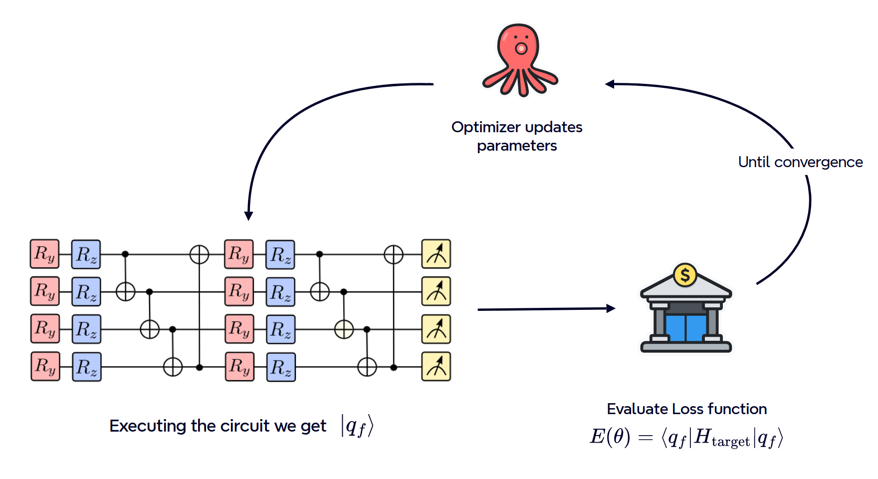
As sketched above, the idea is that we get a state from a quantum circuit, and this state depends on the parameters of the circuit. Then we implement a machine learning routine to update the parameters of the circuit such that the expectation value of our target Hamiltonian on this state is minimized.

Some imports

import numpy as np

import torch.optim as optim

from qibo import (
    Circuit,
    gates,
    hamiltonians,
    set_backend,
    construct_backend,
)

from qiboml.models.decoding import Expectation
from qiboml.interfaces.pytorch import QuantumModel

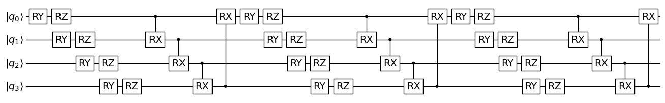
The chosen model

We choose a layered model, where a parametric structure composed of rotations and controlled rotations is repeated nlayers times.

# Setting number of qubits of the problem and number of layers.
nqubits = 4
nlayers = 3

# Structure of the VQE ansatz
def build_vqe_circuit(nqubits, nlayers):
    """Construct a layered, trainable ansatz."""
    c = Circuit(nqubits)
    for _ in range(nlayers):
        for q in range(nqubits):
            c.add(gates.RY(q=q, theta=np.random.randn()))
            c.add(gates.RZ(q=q, theta=np.random.randn()))
        [c.add(gates.CRX(q0=q%nqubits, q1=(q+1)%nqubits, theta=np.random.randn())) for q in range(nqubits)]
    return c

Choice of the target

As target, we select a one-dimensional Heisenberg Hamiltonian with gap set to \(\Delta=0.5\).

# Define the target Hamiltonian
set_backend("qiboml", platform="pytorch")
hamiltonian = hamiltonians.XXZ(nqubits=nqubits, delta=0.5)

[Qibo 0.2.18|INFO|2025-05-19 18:24:38]: Using qiboml (pytorch) backend on cpu

This choice has to be provided to our decoding layer. In fact, our loss function will be exactly the output of this decoding: the expectation value of the given observable (the target Hamiltonian) over the final state prepared by the quantum model.

# Construct the decoding layer
decoding = Expectation(
    nqubits=nqubits,
    observable=hamiltonian,
)

Building the whole model

Our quantum model will present a circuit structure corresponding to our layered ansatz and an expectation value as decoding strategy.

model = QuantumModel(
    circuit_structure=build_vqe_circuit(nqubits=nqubits, nlayers=nlayers),
    decoding=decoding,
)

_ = model.draw()

Let’s train!

print("Exact ground state: ", min(hamiltonian.eigenvalues()))

Exact ground state:  tensor(-6.7446, dtype=torch.float64)

optimizer = optim.Adam(model.parameters(), lr=0.05)

for iteration in range(300):
    optimizer.zero_grad()
    cost = model()
    cost.backward()
    optimizer.step()

    if iteration % 20 == 0:
        print(f"Iteration {iteration}: Cost = {cost.item():.6f}")

Iteration 0: Cost = -0.471007
Iteration 20: Cost = -5.387961
Iteration 40: Cost = -5.990623
Iteration 60: Cost = -6.153267
Iteration 80: Cost = -6.369555
Iteration 100: Cost = -6.604546
Iteration 120: Cost = -6.710510
Iteration 140: Cost = -6.738690
Iteration 160: Cost = -6.743156
Iteration 180: Cost = -6.743962
Iteration 200: Cost = -6.744113
Iteration 220: Cost = -6.744190
Iteration 240: Cost = -6.744234
Iteration 260: Cost = -6.744262
Iteration 280: Cost = -6.744281

We got it 🥳 !